SSF Formulations

Author

Scott Forrest

Published

August 25, 2026

Abstract

In this script we demonstrate different approaches to including covariates in an SSF model.

Load required packages

Code

library(tidyverse)
packages <- c("amt", "sf", "terra", "RColorBrewer", "mgcv", "gratia")
walk(packages, require, character.only = T)

Import data and clean

Code

buffalo_data <- read_csv("data/buffalo.csv")

New names:
Rows: 133161 Columns: 11
── Column specification
──────────────────────────────────────────────────────── Delimiter: "," chr
(2): node, dates dbl (7): ...1, lat, lon, height, accuracy, heading, speed dttm
(2): timestamp, DateTime
ℹ Use `spec()` to retrieve the full column specification for this data. ℹ
Specify the column types or set `show_col_types = FALSE` to quiet this message.
• `` -> `...1`

Code

# remove individuals that have poor data quality or less than about 3 months of data. 
# The "2014.GPS_COMPACT copy.csv" string is a duplicate of ID 2024, so we exclude it
buffalo_data <- buffalo_data %>% filter(!node %in% c("2014.GPS_COMPACT copy.csv", 
                                           2029, 2043, 2265, 2284, 2346))

buffalo_data <- buffalo_data %>%  
  group_by(node) %>% 
  arrange(DateTime, .by_group = T) %>% 
  distinct(DateTime, .keep_all = T) %>% 
  arrange(node) %>% 
  mutate(ID = node)

buffalo_clean <- buffalo_data[, c(12, 2, 4, 3)]
colnames(buffalo_clean) <- c("id", "time", "lon", "lat")
attr(buffalo_clean$time, "tzone") <- "Australia/Queensland"
buffalo_clean$sex <- "f"
buffalo_clean$life_stage <- "adult"
head(buffalo_clean)

Code

tz(buffalo_clean$time)

[1] "Australia/Queensland"

Code

buffalo_ids <- unique(buffalo_clean$id)

write_csv(buffalo_clean, "data/buffalo_clean.csv")

Create a step object

Use the amt package to create a trajectory object from the cleaned data.

Create a trajectory object

buffalo_all <- buffalo_clean %>% mk_track(id = id,
                                           lon,
                                           lat, 
                                           time, 
                                           all_cols = T,
                                           crs = 4326) %>% 
  transform_coords(crs_to = 3112, crs_from = 4326) # Transformation to GDA94 / 
# Geoscience Australia Lambert (https://epsg.io/3112)

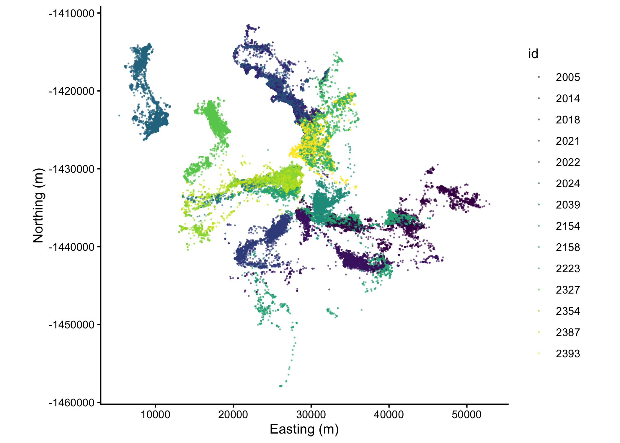
Plot the data spatially

Code

buffalo_all %>%
  ggplot(aes(x = x_, y = y_, colour = id)) +
  geom_point(alpha = 0.5, size = 0.1) + 
  coord_fixed() +
  scale_x_continuous("Easting (m)") +
  scale_y_continuous("Northing (m)") +
  scale_colour_viridis_d() +
  theme_classic() +
  theme(legend.position = "right")

Code

# ggsave("outputs/data_prep/buffalo_djelk_map.png",
#        width = 150, height = 150, units = "mm",  dpi = 600)

Pick out a single individual

Code

which_buffalo <- "2158" # select a single buffalo ID

# create directory to save plots for each buffalo
plot_save_path <- paste0("outputs/buffalo_", which_buffalo)
dir.create(plot_save_path, showWarnings = FALSE)

buffalo_id <- buffalo_all %>% filter(id == which_buffalo)

buffalo_id %>%
  ggplot(aes(x = x_, y = y_, colour = t_)) +
  geom_path(alpha = 0.5) + 
  geom_point(alpha = 0.5, size = 0.1) + 
  coord_fixed() +
  scale_x_continuous("Easting (m)") +
  scale_y_continuous("Northing (m)") +
  theme_classic()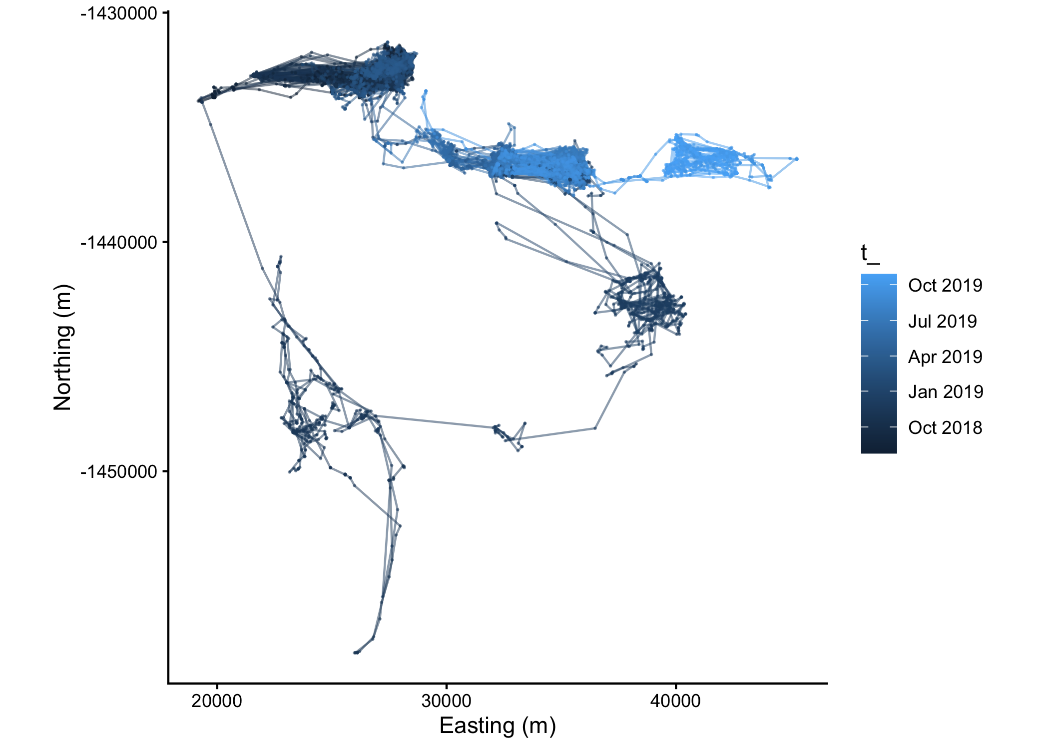

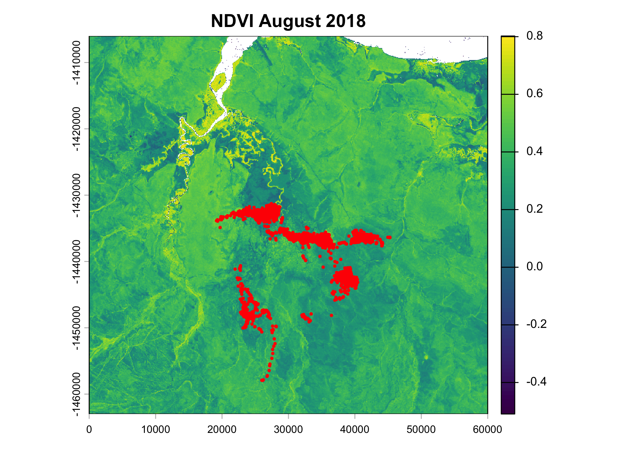
Code

ggsave(paste0(plot_save_path, "/buffalo_id_", which_buffalo, "_map.png"),
       width = 150, height = 150, units = "mm",  dpi = 600)

Import spatial covariate

Although NDVI changes over time, and we have access to monthly layers, we will just select a single month here.

Code

ndvi <- rast("mapping/ndvi_aug_2018.tif")
plot(ndvi, main = "NDVI August 2018")
points(buffalo_id$x_, buffalo_id$y_, col = "red", pch = 16, cex = 0.5)

Code

ndvi

class       : SpatRaster
size        : 2280, 2400, 1  (nrow, ncol, nlyr)
resolution  : 25, 25  (x, y)
extent      : 0, 60000, -1463000, -1406000  (xmin, xmax, ymin, ymax)
coord. ref. : GDA94 / Geoscience Australia Lambert (EPSG:3112)
source      : ndvi_aug_2018.tif
name        :      ndvi
min value   : -0.544105
max value   :  0.808655

Select local extent

We just want to look at an area centred on a single location, which might be combined with our movement probability surface to generate a next-step probability surface.

We’ll centre the extent on an interesting looking part of the landscape, and then buffer it by 1500m (with a buffer of the cell resolution/2 to ensure there is a central cell), which contains most of the step lengths, and therefore most of the movement kernel.

Code

cell_resolution <- 25 # in metres

buffalo_single_point <- buffalo_id[7500,] # select one of the locations

buffer <- 1500 + (cell_resolution/2) # buffer in metres

window_extent <- ext(buffalo_single_point$x_ - buffer, 
                        buffalo_single_point$x_ + buffer, 
                        buffalo_single_point$y_ - buffer, 
                        buffalo_single_point$y_ + buffer)

ndvi_window <- crop(ndvi, window_extent)

# set the extent to 0 at the buffalo location
ndvi_window <- terra::shift(ndvi_window, 
                            dx = -buffalo_single_point$x_, 
                            dy = -buffalo_single_point$y_)

# plot the NDVI layer with the buffalo location as the centre point
plot(ndvi_window, 
     # main = paste0("NDVI"),
     col = brewer.pal(9, "Greens"), 
     plg=list(x="top", title="NDVI", tics="out", cex=.8))
points(x = 0, y = 0, col = "red")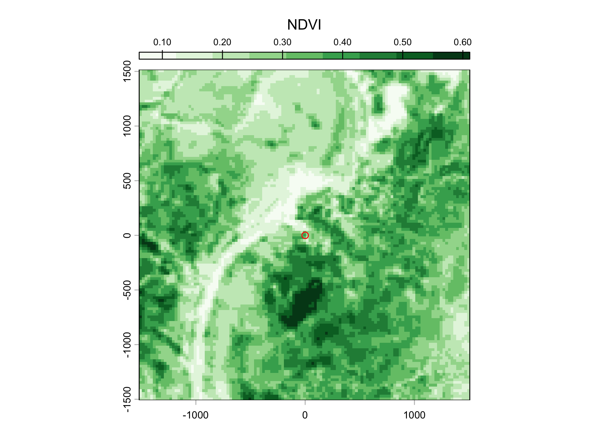

Code

# Save the plot
png(filename = paste0(plot_save_path, "/ndvi_local_", which_buffalo, ".png"), 
    width = 100, height = 100, units = "mm", res = 600)
plot(ndvi_window, 
     # main = paste0("NDVI"),
     col = brewer.pal(9, "Greens"), 
     plg=list(x="top", title="NDVI", tics="out", cex=.8))
points(x = 0, y = 0, col = "red")
dev.off()

quartz_off_screen 
                2

Sample random steps to fit models

Code

buffalo_id_steps <- buffalo_id %>% 
  steps()

# fitting step length and turning angle distributions to all locations
gamma_dist <- fit_distr(buffalo_id_steps$sl_, "gamma")
vonmises_dist <- fit_distr(buffalo_id_steps$ta_, "vonmises")

# movement parameters
gamma_dist$params$shape

[1] 0.4513375

Code

gamma_dist$params$scale

[1] 621.3796

Code

vonmises_dist$params$kappa

[1] 0.1531606

Code

vonmises_dist$params$mu

Circular Data: 
Type = angles 
Units = radians 
Template = none 
Modulo = asis 
Zero = 0 
Rotation = counter 
[1] 0

Code

# sample random steps
buffalo_ssf_data <- buffalo_id_steps %>% 
  random_steps(n = 10, 
                sl_dist = gamma_dist, 
                ta_dist = vonmises_dist) %>%
  extract_covariates(ndvi)  %>%
  mutate(ndvi_sq = ndvi^2,
         log_sl = log(sl_),
         cos_ta = cos(ta_),
         times = 1) # create a dummy column for times (used in a Cox PH model, but not relevant to an SSF) that all contain the same value

Different SSF formulations

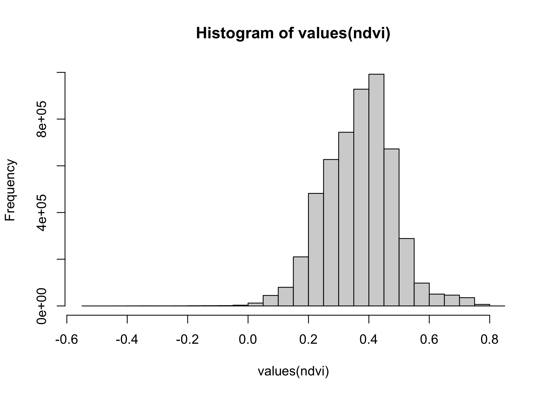
Firstly, we want to pull out the range of NDVI values to plot the curves with.

Code

# histogram of NDVI values
hist(values(ndvi))

Code

# 1% and 99% quantiles of NDVI values
ndvi_quantiles <- quantile(values(ndvi), probs = c(0.005, 0.995), na.rm = TRUE)
ndvi_quantiles

      0.5%      99.5% 
0.06121541 0.71819625

Code

# plot across the range in the local window
ndvi_values <- seq(min(0, ndvi_quantiles[1]), 
                   ndvi_quantiles[2], 
                   length.out = 100)

pred_data <- data.frame(ndvi = ndvi_values, 
                        ndvi_sq = ndvi_values^2,
                        sl_ = 0,
                        log_sl = 0,
                        cos_ta = 0)

Set RSS min and max values

This is hard-coded as the maximum rss value across the different formulations, to ensure the plotting extent is consistent across approaches.

Code

rss_min <- 0
rss_max <- 2.1

Linear covariate

Model formula

\(y \sim ndvi\)

Fit model

Code

# fit an issf model
ssf_linear <- amt::fit_issf(case_ ~ 
                              ndvi + 
                              sl_ + log_sl + cos_ta +
                              strata(step_id_),
                            data = buffalo_ssf_data)

summary(ssf_linear)

Call:
coxph(formula = Surv(rep(1, 106678L), case_) ~ ndvi + sl_ + log_sl + 
    cos_ta + strata(step_id_), data = data, method = "exact")

  n= 106678, number of events= 9698 

             coef  exp(coef)   se(coef)      z Pr(>|z|)    
ndvi   -9.104e-01  4.024e-01  1.444e-01 -6.302 2.93e-10 ***
sl_     1.026e-05  1.000e+00  3.192e-05  0.321    0.748    
log_sl  3.338e-03  1.003e+00  5.687e-03  0.587    0.557    
cos_ta -1.252e-02  9.876e-01  1.503e-02 -0.833    0.405    
---
Signif. codes:  0 '***' 0.001 '**' 0.01 '*' 0.05 '.' 0.1 ' ' 1

       exp(coef) exp(-coef) lower .95 upper .95
ndvi      0.4024     2.4853    0.3032     0.534
sl_       1.0000     1.0000    0.9999     1.000
log_sl    1.0033     0.9967    0.9922     1.015
cos_ta    0.9876     1.0126    0.9589     1.017

Concordance= 0.501  (se = 0.004 )
Likelihood ratio test= 42.36  on 4 df,   p=1e-08
Wald test            = 41.2  on 4 df,   p=2e-08
Score (logrank) test = 41.21  on 4 df,   p=2e-08

Code

AIC(ssf_linear)

[1] 46475.21

Code

# fit an ssf gam model with parametric terms
ssf_linear_gam <- mgcv::gam(cbind(times, step_id_) ~ 
                              ndvi +
                              sl_ + log_sl + cos_ta,
                            data = buffalo_ssf_data,
                            family = cox.ph,
                            weight = case_)

summary(ssf_linear_gam)


Family: Cox PH 
Link function: identity 

Formula:
cbind(times, step_id_) ~ ndvi + sl_ + log_sl + cos_ta

Parametric coefficients:
         Estimate Std. Error z value Pr(>|z|)    
ndvi   -9.104e-01  1.444e-01  -6.302 2.93e-10 ***
sl_     1.026e-05  3.192e-05   0.321    0.748    
log_sl  3.338e-03  5.687e-03   0.587    0.557    
cos_ta -1.252e-02  1.503e-02  -0.833    0.405    
---
Signif. codes:  0 '***' 0.001 '**' 0.01 '*' 0.05 '.' 0.1 ' ' 1


Deviance explained = -0.0499%
-REML =  23252  Scale est. = 1         n = 106678

Code

AIC(ssf_linear_gam)

[1] 46475.21

Code

# Get predictions on log-scale with standard errors
predictions <- predict(ssf_linear_gam, 
                      newdata = pred_data, 
                      type = "link",  # log-scale
                      se.fit = TRUE)

# Extract log RSS and standard errors
log_rss <- predictions$fit
se_log_rss <- predictions$se.fit

# Calculate confidence intervals on log-scale
log_rss_lower <- log_rss - 1.96 * se_log_rss
log_rss_upper <- log_rss + 1.96 * se_log_rss

# Transform to RSS scale
rss <- exp(log_rss)
rss_lower <- exp(log_rss_lower)
rss_upper <- exp(log_rss_upper)

# Create your dataframe
ndvi_coef_df <- data.frame(
  ndvi_values = ndvi_values,
  log_rss = log_rss,
  log_rss_lower = log_rss_lower,
  log_rss_upper = log_rss_upper,
  rss = rss,
  rss_lower = rss_lower,
  rss_upper = rss_upper
)

# plot the response curve
ggplot(data = ndvi_coef_df) +
  geom_hline(yintercept = 1, linetype = "dashed", colour = "grey") +
  geom_ribbon(aes(x = ndvi_values, ymin = rss_lower, ymax = rss_upper), 
              fill = "grey70", alpha = 0.5) +
  geom_line(aes(x = ndvi_values, y = rss), 
            colour = "black", linewidth = 1) +
  scale_x_continuous(breaks = seq(-0.2, 0.8, by = 0.1)) +
  labs(x = "NDVI", y = "RSS") +
  theme_classic()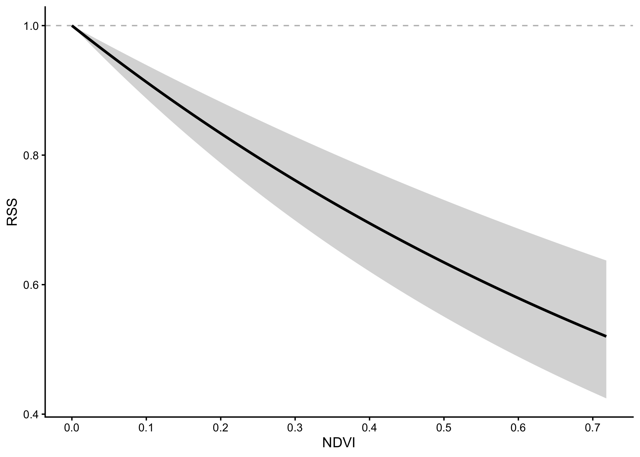

Response curve

Code

# extract the NDVI coefficient and its standard error
ndvi_coef <- ssf_linear$model$coefficients[1]
ndvi_coef_se <- sqrt(diag(ssf_linear$model$var))[1]  # SE of coefficient

# calculate the RSS for each NDVI value
ndvi_coef_df <- data.frame(
  ndvi_values = ndvi_values,
  log_rss = ndvi_values * ndvi_coef,
  rss = exp(ndvi_values * ndvi_coef),
  se_prediction = abs(ndvi_values) * ndvi_coef_se  # SE of prediction at each NDVI value
)

# plot the response curve
ggplot(data = ndvi_coef_df) +
  geom_hline(yintercept = 1, linetype = "dashed", colour = "grey") +
  geom_ribbon(aes(x = ndvi_values, ymin = exp(log_rss - 1.96 * se_prediction), ymax = exp(log_rss + 1.96 * se_prediction)), 
              fill = "grey70", alpha = 0.5) +
  geom_line(aes(x = ndvi_values, y = rss), 
            colour = "black", linewidth = 1) +
  geom_rug(data = buffalo_ssf_data %>% filter(case_ == T), 
           aes(x = ndvi), alpha = 0.25, sides="b") +
  scale_x_continuous(breaks = seq(-0.2, 0.8, by = 0.1)) +
  scale_y_continuous(limits = c(rss_min, rss_max)) +
  labs(x = "NDVI", y = "RSS") +
  theme_classic()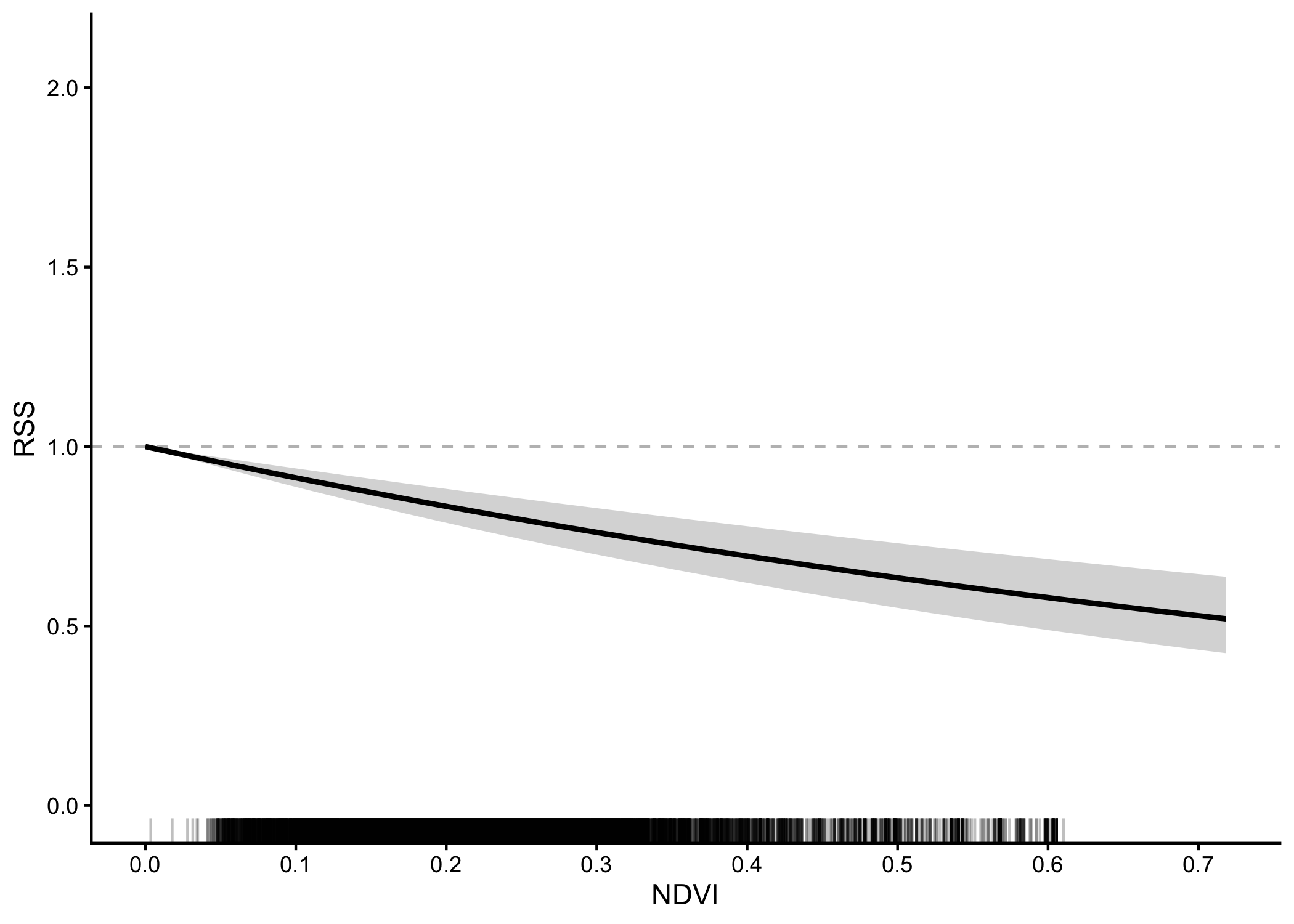

Code

ggsave(paste0(plot_save_path, "/ndvi_linear_response_id", which_buffalo, ".png"),
       width = 120, height = 100, units = "mm", dpi = 600)

Plot habitat selection

Code

# calculate the RSS for the local NDVI values
ndvi_linear <- exp(ndvi_window * ndvi_coef)

# plot the habitat selection (spatial RSS)
plot(ndvi_linear, main = "RSS - linear")

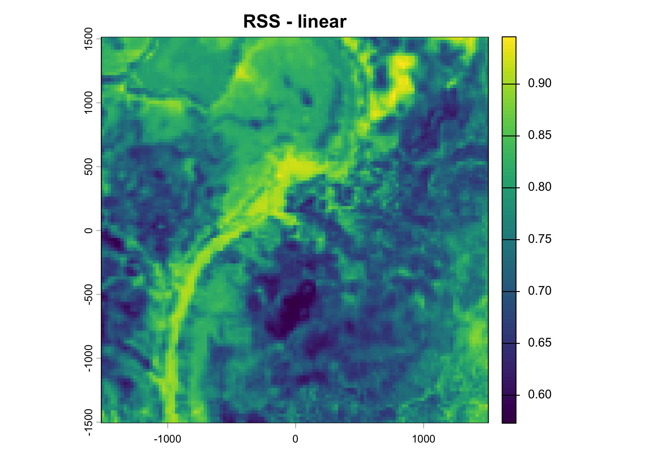
Code

# Save the plot
png(filename = paste0(plot_save_path, "/rss_linear_", which_buffalo, ".png"), 
    width = 100, height = 80, units = "mm", res = 600)
plot(ndvi_linear, main = "RSS - linear", range = c(0.5, 1.75))
dev.off()

quartz_off_screen 
                2

Quadratic covariate

Model formula

\(y \sim ndvi + ndvi^2\)

Fit model

Code

# fit an issf model
ssf_quadratic <- amt::fit_issf(case_ ~ 
                                 ndvi + 
                                 ndvi_sq + 
                                 sl_ + log_sl + cos_ta +
                              strata(step_id_),
                            data = buffalo_ssf_data)

summary(ssf_quadratic)

Call:
coxph(formula = Surv(rep(1, 106678L), case_) ~ ndvi + ndvi_sq + 
    sl_ + log_sl + cos_ta + strata(step_id_), data = data, method = "exact")

  n= 106678, number of events= 9698 

              coef  exp(coef)   se(coef)       z Pr(>|z|)    
ndvi     4.462e+00  8.668e+01  4.981e-01   8.958   <2e-16 ***
ndvi_sq -9.008e+00  1.224e-04  8.157e-01 -11.044   <2e-16 ***
sl_     -8.545e-06  1.000e+00  3.201e-05  -0.267    0.790    
log_sl   7.233e-03  1.007e+00  5.720e-03   1.265    0.206    
cos_ta  -1.353e-02  9.866e-01  1.504e-02  -0.899    0.369    
---
Signif. codes:  0 '***' 0.001 '**' 0.01 '*' 0.05 '.' 0.1 ' ' 1

        exp(coef) exp(-coef) lower .95 upper .95
ndvi    8.668e+01  1.154e-02 3.265e+01 2.301e+02
ndvi_sq 1.224e-04  8.169e+03 2.475e-05 6.055e-04
sl_     1.000e+00  1.000e+00 9.999e-01 1.000e+00
log_sl  1.007e+00  9.928e-01 9.960e-01 1.019e+00
cos_ta  9.866e-01  1.014e+00 9.579e-01 1.016e+00

Concordance= 0.528  (se = 0.003 )
Likelihood ratio test= 175.8  on 5 df,   p=<2e-16
Wald test            = 147.1  on 5 df,   p=<2e-16
Score (logrank) test = 147.2  on 5 df,   p=<2e-16

Code

AIC(ssf_quadratic)

[1] 46343.8

Code

# fit an ssf gam model with parametric terms. -ends up being the same as above, 
# but allows us to use the `predict` function to get predictions on the log-scale with standard errors, 
# which is a bit more work to do with the `amt` model object.
ssf_quadratic_gam <- mgcv::gam(cbind(times, step_id_) ~ 
                                 ndvi + 
                                 ndvi_sq +
                               sl_ + log_sl + cos_ta,
                               data = buffalo_ssf_data,
                               family = cox.ph,
                               weight = case_)

summary(ssf_quadratic_gam)


Family: Cox PH 
Link function: identity 

Formula:
cbind(times, step_id_) ~ ndvi + ndvi_sq + sl_ + log_sl + cos_ta

Parametric coefficients:
          Estimate Std. Error z value Pr(>|z|)    
ndvi     4.462e+00  4.981e-01   8.958   <2e-16 ***
ndvi_sq -9.008e+00  8.157e-01 -11.044   <2e-16 ***
sl_     -8.545e-06  3.201e-05  -0.267    0.790    
log_sl   7.233e-03  5.720e-03   1.265    0.206    
cos_ta  -1.353e-02  1.504e-02  -0.899    0.369    
---
Signif. codes:  0 '***' 0.001 '**' 0.01 '*' 0.05 '.' 0.1 ' ' 1


Deviance explained = -0.0992%
-REML =  23184  Scale est. = 1         n = 106678

Code

AIC(ssf_quadratic_gam)

[1] 46343.8

Generate the response curve

Code

# Get predictions on log-scale with standard errors
predictions <- predict(ssf_quadratic_gam, 
                      newdata = pred_data, 
                      type = "link",  # log-scale
                      se.fit = TRUE)

# Extract log RSS and standard errors
log_rss <- predictions$fit
se_log_rss <- predictions$se.fit

# Calculate confidence intervals on log-scale
log_rss_lower <- log_rss - 1.96 * se_log_rss
log_rss_upper <- log_rss + 1.96 * se_log_rss

# Transform to RSS scale
rss <- exp(log_rss)
rss_lower <- exp(log_rss_lower)
rss_upper <- exp(log_rss_upper)

# Create your dataframe
ndvi_coef_df <- data.frame(
  ndvi_values = ndvi_values,
  log_rss = log_rss,
  log_rss_lower = log_rss_lower,
  log_rss_upper = log_rss_upper,
  rss = rss,
  rss_lower = rss_lower,
  rss_upper = rss_upper
)

# plot the response curve
ggplot(data = ndvi_coef_df) +
  geom_hline(yintercept = 1, linetype = "dashed", colour = "grey") +
  geom_ribbon(aes(x = ndvi_values, ymin = rss_lower, ymax = rss_upper), 
              fill = "grey70", alpha = 0.5) +
  geom_line(aes(x = ndvi_values, y = rss), 
            colour = "black", linewidth = 1) +
  geom_rug(data = buffalo_ssf_data %>% filter(case_ == T), 
           aes(x = ndvi), alpha = 0.25, sides="b") +
  scale_x_continuous(breaks = seq(-0.2, 0.8, by = 0.1)) +
  scale_y_continuous(limits = c(rss_min, rss_max)) +
  labs(x = "NDVI", y = "RSS") +
  theme_classic()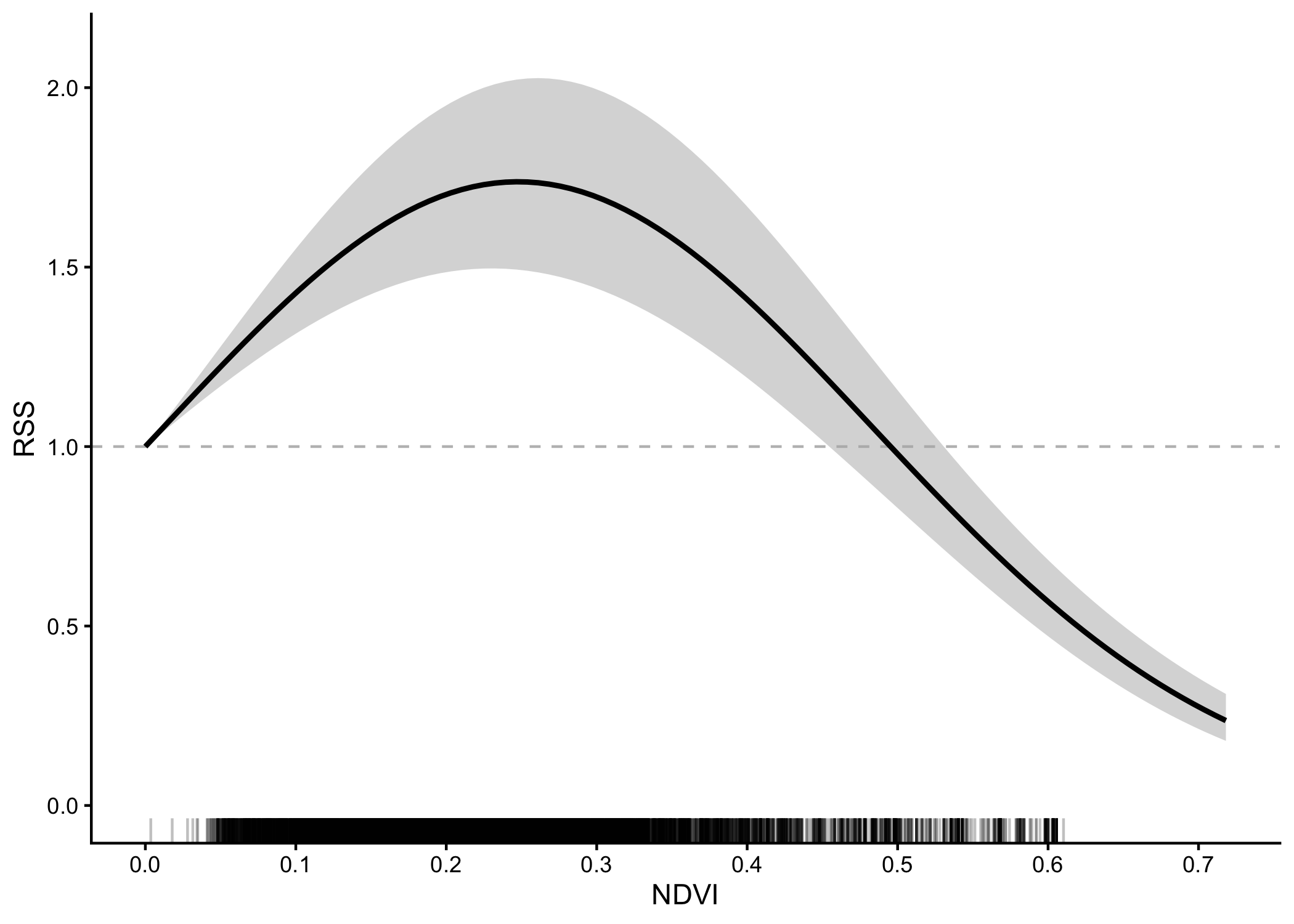

Code

ggsave(paste0(plot_save_path, "/ndvi_quadratic_response_id", which_buffalo, ".png"),
       width = 120, height = 100, units = "mm", dpi = 600)

Response curve

Code

# extract the NDVI coefficient
ndvi_coef <- ssf_quadratic$model$coefficients[1]
ndvi_coef_sq <- ssf_quadratic$model$coefficients[2]

ndvi_se = sqrt(diag(ssf_quadratic$model$var))[1]
ndvi_sq_se = sqrt(diag(ssf_quadratic$model$var))[2]

log_rss = (ndvi_values * ndvi_coef) + (ndvi_values^2 * ndvi_coef_sq)
rss = exp(log_rss)

# calculate the RSS for each NDVI value
ndvi_coef_df <- data.frame(ndvi_values, log_rss, rss)

# plot the response curve
ggplot() +
  geom_hline(yintercept = 1, linetype = "dashed", colour = "grey") +
  geom_line(data = ndvi_coef_df, aes(x = ndvi_values, y = rss), 
            colour = "black", linewidth = 1) +
  scale_x_continuous(breaks = seq(-0.2, 0.8, by = 0.1)) +
  labs(x = "NDVI", y = "RSS") +
  theme_classic()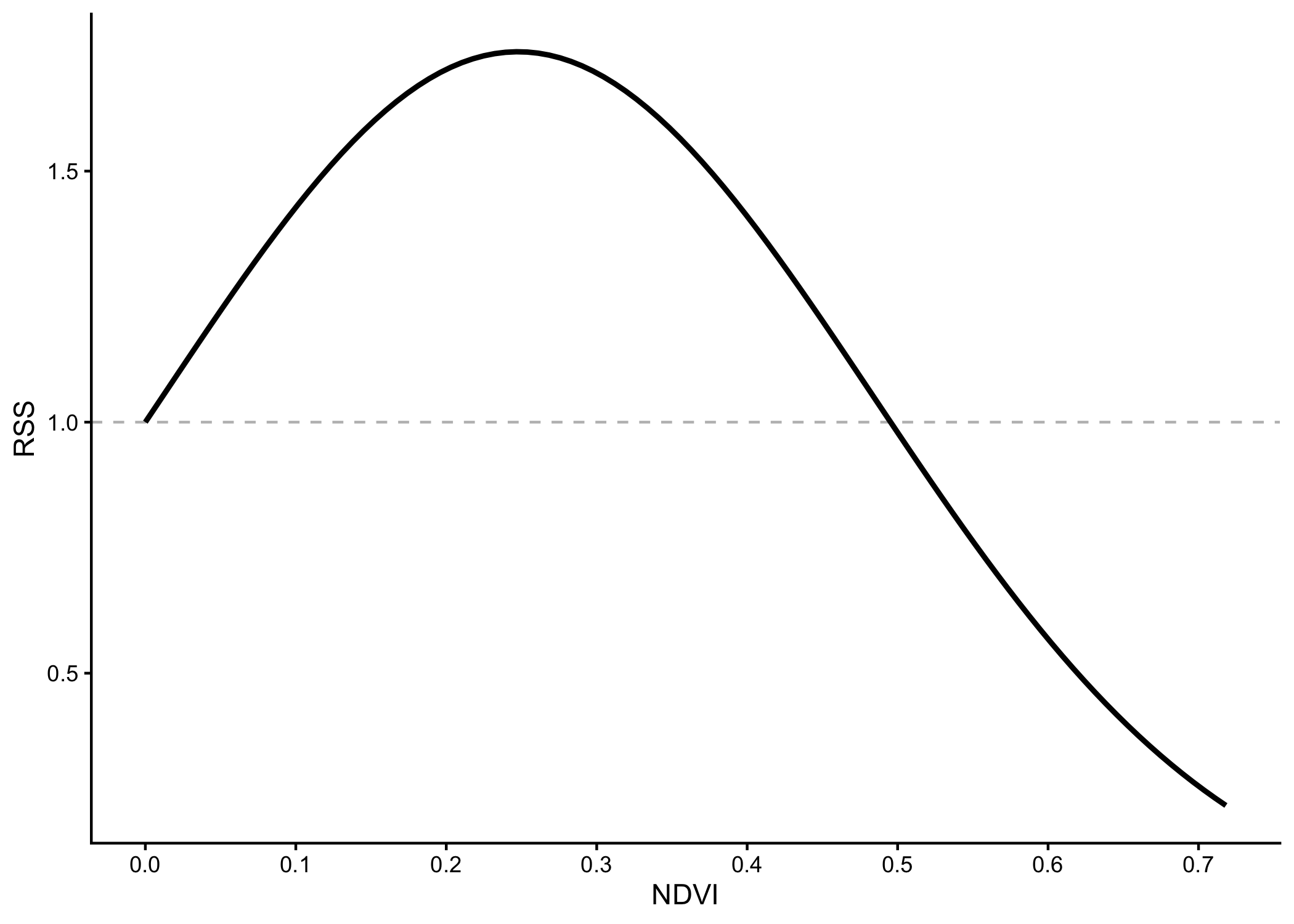

Code

# ggsave(paste0(plot_save_path, /ndvi_quadratic_response_id", which_buffalo, ".png"),
#        width = 100, height = 100, units = "mm", dpi = 600)

Plot habitat selection

Code

# extract the NDVI coefficient
ndvi_coef <- ssf_quadratic$model$coefficients[1]
ndvi_coef_sq <- ssf_quadratic$model$coefficients[2]

# calculate the RSS for the local NDVI values
ndvi_quadratic <- exp((ndvi_window * ndvi_coef) + 
                        (ndvi_window^2 * ndvi_coef_sq))

# plot the habitat selection (spatial RSS)
plot(ndvi_quadratic, main = "RSS - quadratic")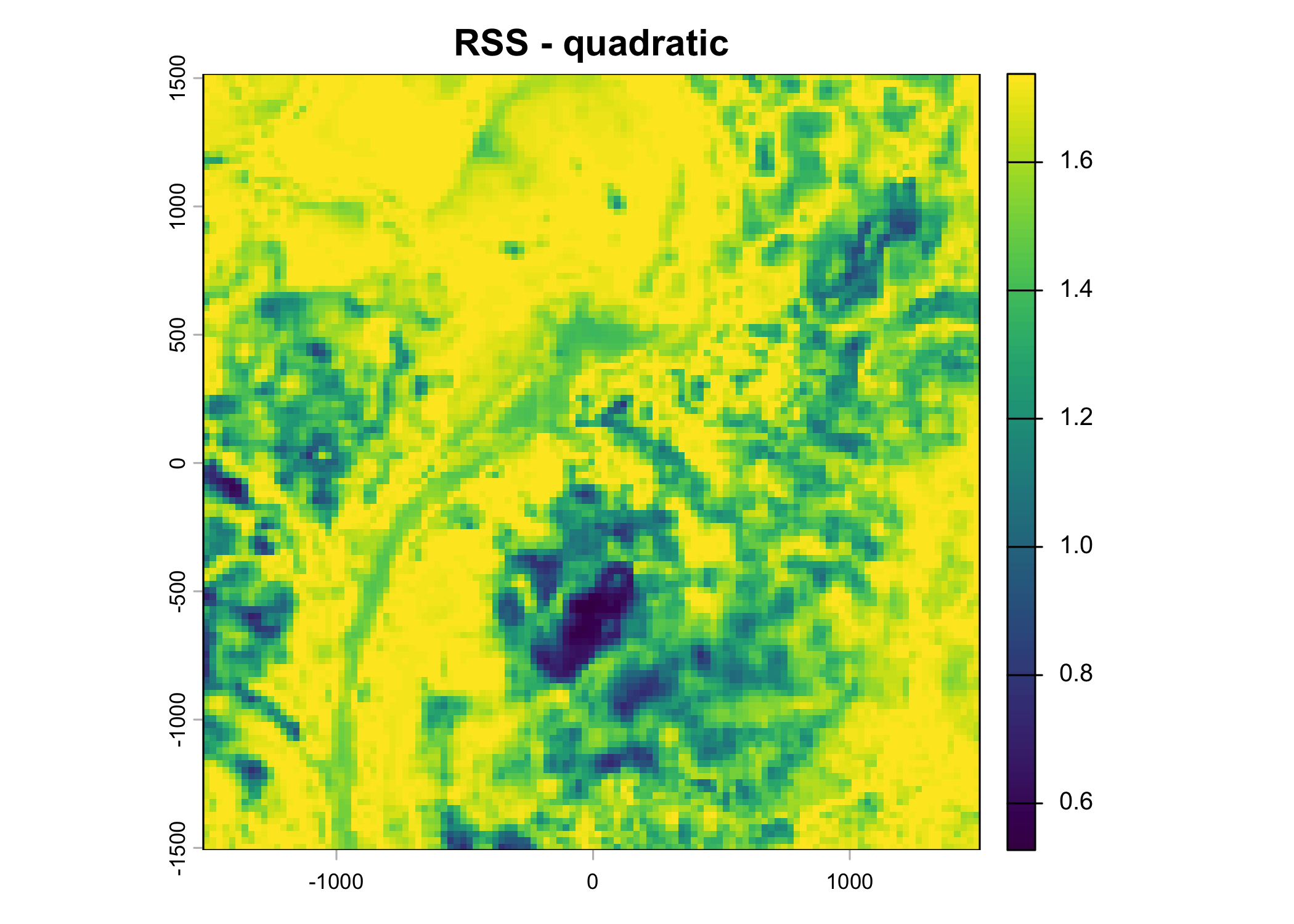

Code

# Save the plot
png(filename = paste0(plot_save_path, "/rss_quadratic_", which_buffalo, ".png"), 
    width = 100, height = 80, units = "mm", res = 600)
plot(ndvi_quadratic, main = "RSS - quadratic", range = c(0.5, 1.75))
dev.off()

quartz_off_screen 
                2

Smooth term

Fit a GAM to the data, with a smooth term across the range of NDVI values (Klappstein et al. 2024).

Model formula

\(y \sim s(ndvi)\)

Fit model

Code

# fit an ssf gam model
ssf_gam <- mgcv::gam(cbind(times, step_id_) ~ 
                       s(ndvi, bs = "cr") + 
                       # s(ndvi) +
                       sl_ + log_sl + cos_ta,
                            data = buffalo_ssf_data,
                            family = cox.ph,
                            weight = case_)

summary(ssf_gam)


Family: Cox PH 
Link function: identity 

Formula:
cbind(times, step_id_) ~ s(ndvi, bs = "cr") + sl_ + log_sl + 
    cos_ta

Parametric coefficients:
         Estimate Std. Error z value Pr(>|z|)  
sl_     1.530e-06  3.196e-05   0.048   0.9618  
log_sl  1.211e-02  5.761e-03   2.102   0.0355 *
cos_ta -1.345e-02  1.506e-02  -0.893   0.3719  
---
Signif. codes:  0 '***' 0.001 '**' 0.01 '*' 0.05 '.' 0.1 ' ' 1

Approximate significance of smooth terms:
          edf Ref.df Chi.sq p-value    
s(ndvi) 8.418   8.85    383  <2e-16 ***
---
Signif. codes:  0 '***' 0.001 '**' 0.01 '*' 0.05 '.' 0.1 ' ' 1

Deviance explained = 0.33%
-REML =  23089  Scale est. = 1         n = 106678

Code

AIC(ssf_gam)

[1] 46120.8

Code

# coef(ssf_gam)[4]

gam_smooths <- gratia::smooth_estimates(ssf_gam)

Using ggplot with the smooth_estimates dataframe from gratia

Code

ggplot(data = gam_smooths) + 
  geom_hline(yintercept = 1, linetype = "dashed", colour = "grey") +
  geom_ribbon(aes(x = ndvi, ymin = exp(.estimate - 1.96 * .se), ymax = exp(.estimate + 1.96 * .se)), 
              fill = "grey70", alpha = 0.5) +
  geom_line(aes(x = ndvi, y = exp(.estimate)), 
            colour = "black", linewidth = 1) +
  labs(x = "NDVI", y = "RSS") +
  # scale_x_continuous(limits = c(ndvi_quantiles[1], 0.5)) +
  # scale_y_continuous(limits = c(0.65, 1.3)) +
  theme_classic()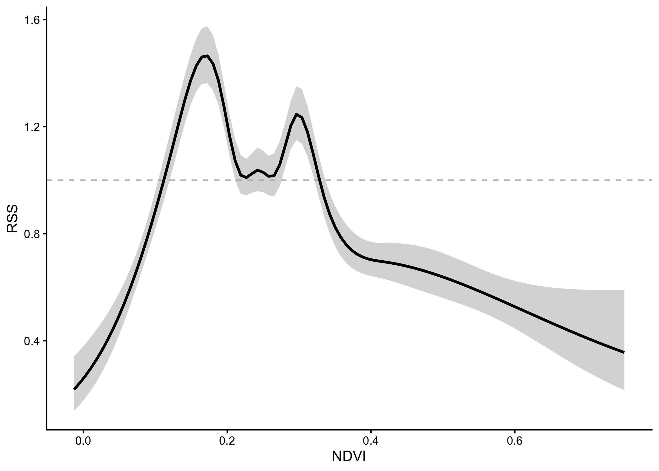

Code

ggsave(paste0(plot_save_path, "/ndvi_smooth_response_id", which_buffalo, ".png"),
       width = 120, height = 100, units = "mm", dpi = 600)

ALternatively, generate the response curve with the `predict` function

Code

# Get predictions on log-scale with standard errors
predictions <- predict(ssf_gam, 
                      newdata = pred_data, 
                      type = "link",  # log-scale
                      se.fit = TRUE)

# Extract log RSS and standard errors
log_rss <- predictions$fit
se_log_rss <- predictions$se.fit

# Calculate confidence intervals on log-scale
log_rss_lower <- log_rss - 1.96 * se_log_rss
log_rss_upper <- log_rss + 1.96 * se_log_rss

# Transform to RSS scale
rss <- exp(log_rss)
rss_lower <- exp(log_rss_lower)
rss_upper <- exp(log_rss_upper)

# Create your dataframe
ndvi_coef_df <- data.frame(
  ndvi_values = ndvi_values,
  log_rss = log_rss,
  log_rss_lower = log_rss_lower,
  log_rss_upper = log_rss_upper,
  rss = rss,
  rss_lower = rss_lower,
  rss_upper = rss_upper
)

# plot the response curve
ggplot(data = ndvi_coef_df) +
  geom_hline(yintercept = 1, linetype = "dashed", colour = "grey") +
  geom_ribbon(aes(x = ndvi_values, ymin = rss_lower, ymax = rss_upper), 
              fill = "grey70", alpha = 0.5) +
  geom_line(aes(x = ndvi_values, y = rss), 
            colour = "black", linewidth = 1) +
  geom_rug(data = buffalo_ssf_data %>% filter(case_ == T), 
           aes(x = ndvi), alpha = 0.25, sides="b") +
  scale_x_continuous(breaks = seq(-0.2, 0.8, by = 0.1)) +
  scale_y_continuous(limits = c(rss_min, rss_max)) +
  labs(x = "NDVI", y = "RSS") +
  theme_classic()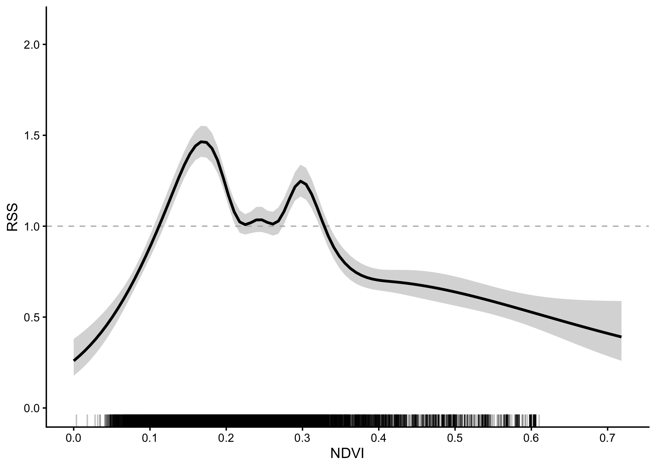

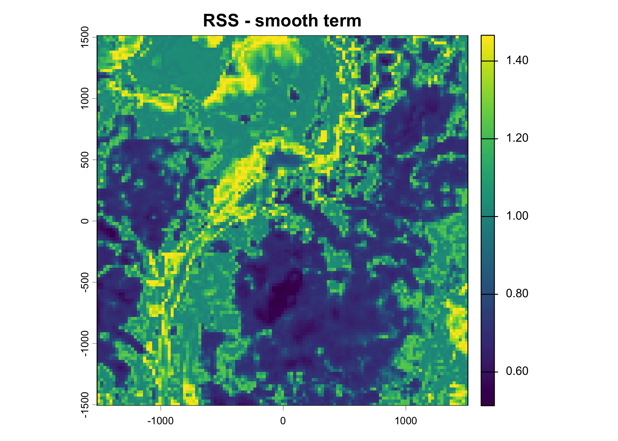
Code

ggsave(paste0(plot_save_path, "/ndvi_smooth_response_id", which_buffalo, ".png"),
       width = 120, height = 100, units = "mm", dpi = 600)

Plot habitat selection

Code

predicted_log_rss <- predict(ssf_gam, 
                         newdata = data.frame(ndvi = values(ndvi_window), 
                                                sl_ = 0, 
                                                log_sl = 0, 
                                                cos_ta = 0),, 
                         type = "link")

ndvi_gam <- ndvi_window
values(ndvi_gam) <- exp(as.vector(predicted_log_rss))

# Plot the predictions
plot(ndvi_gam, main = "RSS - smooth term")

Code

# Save the plot
png(filename = paste0(plot_save_path, "/rss_smooth_", which_buffalo, ".png"), 
    width = 100, height = 80, units = "mm", res = 600)
plot(ndvi_gam, main = "RSS - smooth", range = c(0.5, 1.75))
dev.off()

quartz_off_screen 
                2

Temporal dynamics

Static model for comparison

Code

ssf_static <- amt::fit_issf(case_ ~ 
                                 ndvi +sl_ + log_sl + cos_ta +
                                 strata(step_id_),
                               data = buffalo_ssf_data)

summary(ssf_static)

Call:
coxph(formula = Surv(rep(1, 106678L), case_) ~ ndvi + sl_ + log_sl + 
    cos_ta + strata(step_id_), data = data, method = "exact")

  n= 106678, number of events= 9698 

             coef  exp(coef)   se(coef)      z Pr(>|z|)    
ndvi   -9.104e-01  4.024e-01  1.444e-01 -6.302 2.93e-10 ***
sl_     1.026e-05  1.000e+00  3.192e-05  0.321    0.748    
log_sl  3.338e-03  1.003e+00  5.687e-03  0.587    0.557    
cos_ta -1.252e-02  9.876e-01  1.503e-02 -0.833    0.405    
---
Signif. codes:  0 '***' 0.001 '**' 0.01 '*' 0.05 '.' 0.1 ' ' 1

       exp(coef) exp(-coef) lower .95 upper .95
ndvi      0.4024     2.4853    0.3032     0.534
sl_       1.0000     1.0000    0.9999     1.000
log_sl    1.0033     0.9967    0.9922     1.015
cos_ta    0.9876     1.0126    0.9589     1.017

Concordance= 0.501  (se = 0.004 )
Likelihood ratio test= 42.36  on 4 df,   p=1e-08
Wald test            = 41.2  on 4 df,   p=2e-08
Score (logrank) test = 41.21  on 4 df,   p=2e-08

Code

AIC(ssf_static)

[1] 46475.21

Code

ndvi_coef <- ssf_static$model$coefficients["ndvi"]
ndvi_se <- sqrt(diag(ssf_static$model$var))[1]  # SE of coefficient

ndvi_static_coef_df <- data.frame(hour = seq(0, 23, length.out = 231),
                                    ndvi_coef = ndvi_coef,
                                    ndvi_se = ndvi_se,
                                    ndvi_lo = ndvi_coef - 1.96 * ndvi_se,
                                    ndvi_hi = ndvi_coef + 1.96 * ndvi_se)

Warning in data.frame(hour = seq(0, 23, length.out = 231), ndvi_coef =
ndvi_coef, : row names were found from a short variable and have been discarded

Code

# Plot with ribbon
ggplot(ndvi_static_coef_df, aes(x = hour)) +
  geom_hline(yintercept = 0, linetype = "dashed", colour = "black") +
  geom_vline(xintercept = 9, linetype = "dashed", colour = "orange") +
  geom_vline(xintercept = 17, linetype = "dashed", colour = "skyblue") +
  geom_ribbon(aes(ymin = ndvi_lo, ymax = ndvi_hi), alpha = 0.2) +
  geom_line(aes(y = ndvi_coef)) +
  labs(title = "ndvi", x = "Hour", y = expression(beta[NDVI]), fill = NULL) +
  scale_x_continuous(breaks = seq(0, 24, by = 4)) +
  scale_y_continuous(limits = c(-5,3.5), breaks = seq(-5, 4, by = 1)) +
  theme_classic()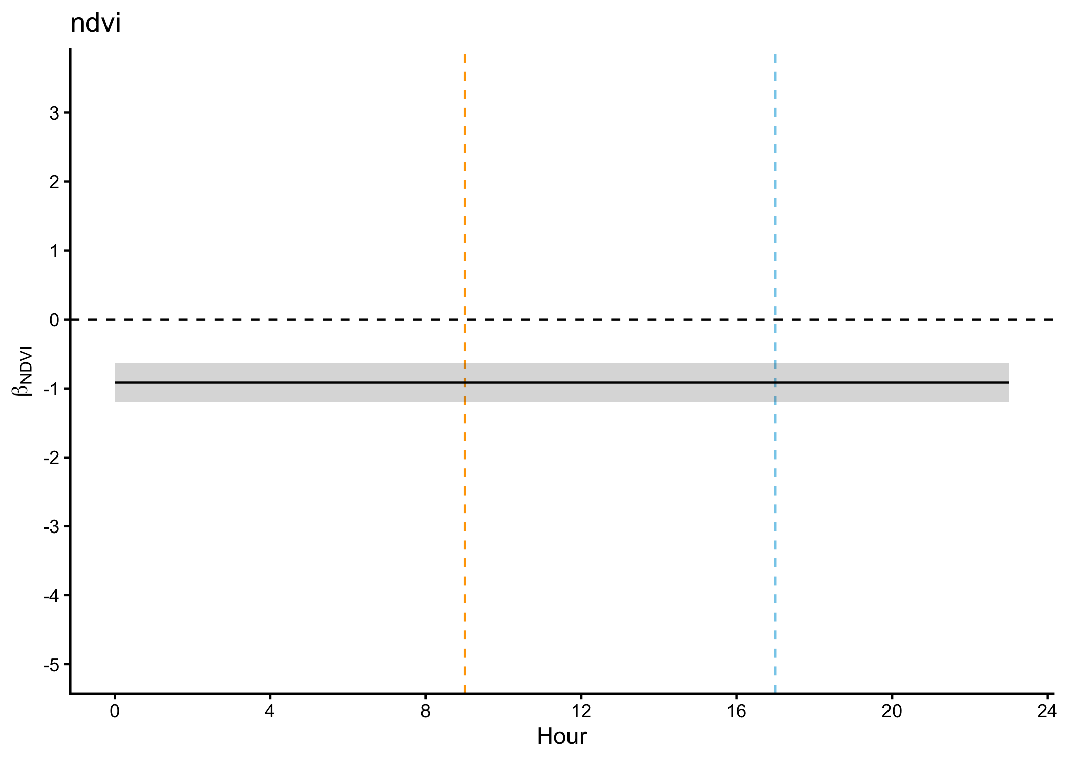

Code

ggsave(paste0(plot_save_path, "/ndvi_static_coef_response_id", which_buffalo, ".png"),
       width = 150, height = 80, units = "mm", dpi = 600)

Pull out a response curve from one of the hours

Code

sample_hours <- c(9, 17)

ndvi_coef_df <- purrr::map_dfr(sample_hours, function(sample_hour) {
  
  # extract the NDVI coefficient and its standard error
  ndvi_coef <- ndvi_static_coef_df %>% filter(hour == sample_hour) %>% pull(ndvi_coef)
  ndvi_coef_se <- ndvi_static_coef_df %>% filter(hour == sample_hour) %>% pull(ndvi_se)
  
  # calculate the RSS for each NDVI value
  data.frame(
    ndvi_values = ndvi_values,
    log_rss = ndvi_values * ndvi_coef,
    rss = exp(ndvi_values * ndvi_coef),
    se_prediction = abs(ndvi_values) * ndvi_coef_se
  ) %>% mutate(hour = as.factor(sample_hour), .before = ndvi_values)
  
})

# plot the response curve
ggplot(data = ndvi_coef_df) +
  geom_hline(yintercept = 1, linetype = "dashed", colour = "grey") +
  geom_ribbon(aes(x = ndvi_values, 
                  ymin = exp(log_rss - 1.96 * se_prediction), 
                  ymax = exp(log_rss + 1.96 * se_prediction),
                  fill = hour), 
              alpha = 0.5) +
  geom_line(aes(x = ndvi_values, y = rss, colour = hour), 
            linewidth = 1) +
  geom_rug(data = buffalo_ssf_data %>% filter(case_ == T), 
           aes(x = ndvi), alpha = 0.25, sides="b") +
  scale_colour_manual(values = c("orange", "skyblue")) +
  scale_fill_manual(values = c("orange", "skyblue")) +
  scale_x_continuous(breaks = seq(-0.2, 0.8, by = 0.1)) +
  scale_y_continuous(limits = c(0, 5.5)) +
  labs(x = "NDVI", y = "RSS") +
  theme_classic() +
  theme(legend.position = "none")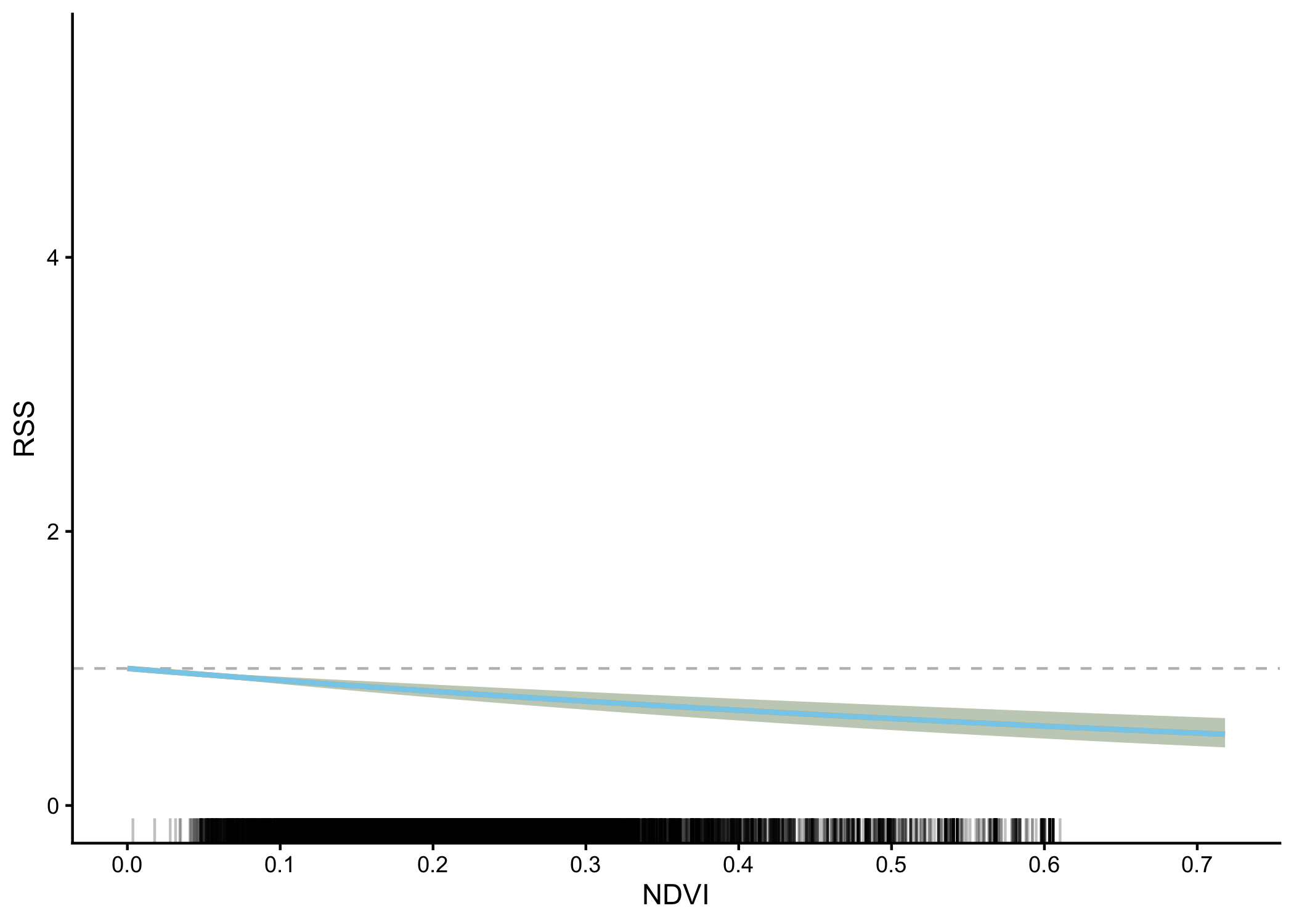

Code

ggsave(paste0(plot_save_path, "/ndvi_static_response_sample_hour_id", which_buffalo, ".png"),
       width = 70, height = 80, units = "mm", dpi = 600)

Fit harmonic model with quadratic terms

Code

ssf_static_quadratic <- amt::fit_issf(case_ ~ 
                                 # linear term
                                 ndvi + 
                                 # quadratic terms
                                 ndvi_sq +
                                 sl_ + log_sl + cos_ta +
                                 strata(step_id_),
                               data = buffalo_ssf_data)

summary(ssf_static_quadratic)

Call:
coxph(formula = Surv(rep(1, 106678L), case_) ~ ndvi + ndvi_sq + 
    sl_ + log_sl + cos_ta + strata(step_id_), data = data, method = "exact")

  n= 106678, number of events= 9698 

              coef  exp(coef)   se(coef)       z Pr(>|z|)    
ndvi     4.462e+00  8.668e+01  4.981e-01   8.958   <2e-16 ***
ndvi_sq -9.008e+00  1.224e-04  8.157e-01 -11.044   <2e-16 ***
sl_     -8.545e-06  1.000e+00  3.201e-05  -0.267    0.790    
log_sl   7.233e-03  1.007e+00  5.720e-03   1.265    0.206    
cos_ta  -1.353e-02  9.866e-01  1.504e-02  -0.899    0.369    
---
Signif. codes:  0 '***' 0.001 '**' 0.01 '*' 0.05 '.' 0.1 ' ' 1

        exp(coef) exp(-coef) lower .95 upper .95
ndvi    8.668e+01  1.154e-02 3.265e+01 2.301e+02
ndvi_sq 1.224e-04  8.169e+03 2.475e-05 6.055e-04
sl_     1.000e+00  1.000e+00 9.999e-01 1.000e+00
log_sl  1.007e+00  9.928e-01 9.960e-01 1.019e+00
cos_ta  9.866e-01  1.014e+00 9.579e-01 1.016e+00

Concordance= 0.528  (se = 0.003 )
Likelihood ratio test= 175.8  on 5 df,   p=<2e-16
Wald test            = 147.1  on 5 df,   p=<2e-16
Score (logrank) test = 147.2  on 5 df,   p=<2e-16

Code

AIC(ssf_static_quadratic)

[1] 46343.8

Create table of NDVI and hour values

Code

ndvi_hour_values <- expand.grid(ndvi = ndvi_values, 
                                hour = seq(0, 23, length.out = length(ndvi_values)))

ndvi_lin_coef <- ssf_static_quadratic$model$coefficients["ndvi"]
ndvi_quad_coef <- ssf_static_quadratic$model$coefficients["ndvi_sq"]

ndvi_hour_values <- ndvi_hour_values %>% mutate(
  ndvi_lin_coef = ndvi_lin_coef,
  ndvi_quad_coef = ndvi_quad_coef,
  ssf_quadratic_log_rss = (ndvi * ndvi_lin_coef) + (ndvi^2 * ndvi_quad_coef)
)


max_abs_colour <- max(abs(range(ndvi_hour_values$ssf_quadratic_log_rss)))

# plot the selection surface
ggplot() +
  geom_raster(data = ndvi_hour_values,
       aes(x = hour, y = ndvi, fill = ssf_quadratic_log_rss)) +
  labs(title = "(ndvi + ndvi^2)", x = "Hour", y = "NDVI", fill = "log-RSS") +
  geom_contour(data = ndvi_hour_values,
       aes(x = hour, y = ndvi, z = ssf_quadratic_log_rss), 
       colour = "black") +
  geom_contour(data = ndvi_hour_values,
       aes(x = hour, y = ndvi, z = ssf_quadratic_log_rss),
       breaks = 0, colour = "black", linetype = "solid", linewidth = 0.75) +
  geom_vline(xintercept = 9, linetype = "dashed", colour = "orange") +
  geom_vline(xintercept = 17, linetype = "dashed", colour = "skyblue") +
  scale_fill_distiller(palette = "RdBu", type = "div", direction = 1,
                       limits = c(-max_abs_colour, max_abs_colour)) +
  coord_cartesian(expand = FALSE) +
  geom_rug(data = buffalo_ssf_data %>% filter(case_ == T),
           aes(y = ndvi), alpha = 0.25, length = unit(0.015, "npc"), sides="l") +
  scale_y_continuous(breaks = seq(-0.2, 0.8, by = 0.1)) +
  theme_bw()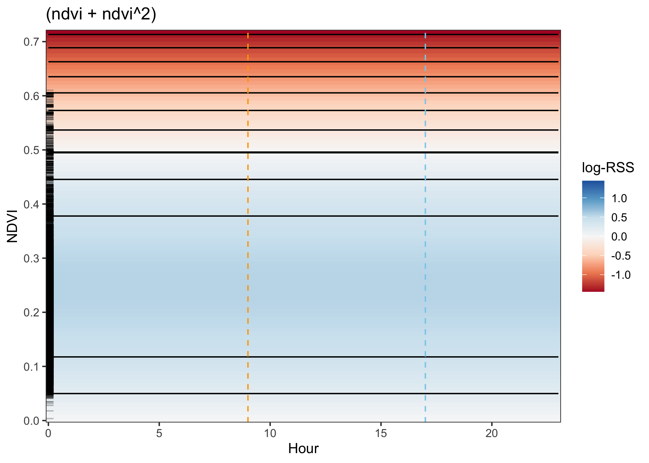

Code

ggsave(paste0(plot_save_path, "/ndvi_static_quadratic_response_id", which_buffalo, ".png"),
       width = 150, height = 80, units = "mm", dpi = 600)

Easier to get the curves with GAM predict function

Fit model

Code

# fit an ssf gam model with parametric terms. -ends up being the same as above, 
# but allows us to use the `predict` function to get predictions on the log-scale with standard errors, 
# which is a bit more work to do with the `amt` model object.
ssf_quadratic_gam <- mgcv::gam(cbind(times, step_id_) ~ 
                                 ndvi + 
                                 ndvi_sq +
                               sl_ + log_sl + cos_ta,
                               data = buffalo_ssf_data,
                               family = cox.ph,
                               weight = case_)

summary(ssf_quadratic_gam)


Family: Cox PH 
Link function: identity 

Formula:
cbind(times, step_id_) ~ ndvi + ndvi_sq + sl_ + log_sl + cos_ta

Parametric coefficients:
          Estimate Std. Error z value Pr(>|z|)    
ndvi     4.462e+00  4.981e-01   8.958   <2e-16 ***
ndvi_sq -9.008e+00  8.157e-01 -11.044   <2e-16 ***
sl_     -8.545e-06  3.201e-05  -0.267    0.790    
log_sl   7.233e-03  5.720e-03   1.265    0.206    
cos_ta  -1.353e-02  1.504e-02  -0.899    0.369    
---
Signif. codes:  0 '***' 0.001 '**' 0.01 '*' 0.05 '.' 0.1 ' ' 1


Deviance explained = -0.0992%
-REML =  23184  Scale est. = 1         n = 106678

Code

AIC(ssf_quadratic_gam)

[1] 46343.8

Generate the response curve

Code

# Get predictions on log-scale with standard errors
predictions <- predict(ssf_quadratic_gam, 
                      newdata = pred_data, 
                      type = "link",  # log-scale
                      se.fit = TRUE)

# Extract log RSS and standard errors
log_rss <- predictions$fit
se_log_rss <- predictions$se.fit

# Calculate confidence intervals on log-scale
log_rss_lower <- log_rss - 1.96 * se_log_rss
log_rss_upper <- log_rss + 1.96 * se_log_rss

# Transform to RSS scale
rss <- exp(log_rss)
rss_lower <- exp(log_rss_lower)
rss_upper <- exp(log_rss_upper)

# Create your dataframe
ndvi_coef_df <- data.frame(
  ndvi_values = ndvi_values,
  log_rss = log_rss,
  log_rss_lower = log_rss_lower,
  log_rss_upper = log_rss_upper,
  rss = rss,
  rss_lower = rss_lower,
  rss_upper = rss_upper
)

ndvi_coef_df <- rbind(data.frame(hour = 9, ndvi_coef_df), data.frame(hour = 17, ndvi_coef_df))

# plot the response curve
ggplot(data = ndvi_coef_df) +
  geom_hline(yintercept = 1, linetype = "dashed", colour = "grey") +
  geom_ribbon(aes(x = ndvi_values, ymin = rss_lower, ymax = rss_upper, fill = as.factor(hour)), 
              alpha = 0.5) +
  geom_line(aes(x = ndvi_values, y = rss, colour = as.factor(hour)), 
            linewidth = 1) +
  geom_rug(data = buffalo_ssf_data %>% filter(case_ == T), 
           aes(x = ndvi), alpha = 0.25, sides="b") +
  scale_colour_manual(values = c("orange", "skyblue")) +
  scale_fill_manual(values = c("orange", "skyblue")) +
  scale_x_continuous(breaks = seq(-0.2, 0.8, by = 0.1)) +
  scale_y_continuous(limits = c(0, 5.5)) +
  labs(x = "NDVI", y = "RSS") +
  theme_classic()  +
  theme(legend.position = "none")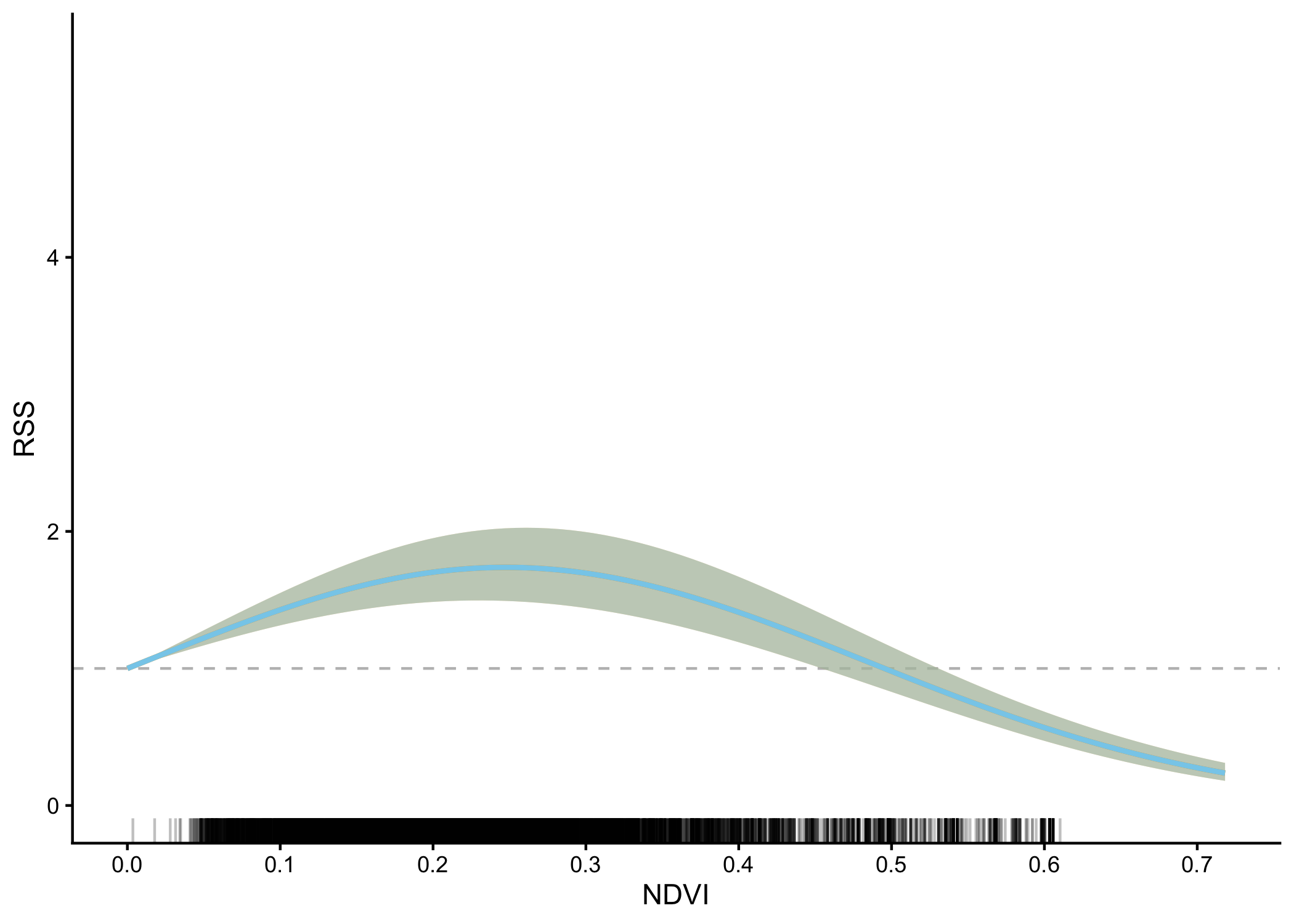

Code

ggsave(paste0(plot_save_path, "/ndvi_static_quadratic_response_sample_hour_id", which_buffalo, ".png"),
       width = 70, height = 80, units = "mm", dpi = 600)

Harmonic regression

Code

buffalo_ssf_data <- buffalo_ssf_data %>% mutate(
  
  # create hour term
  hour = lubridate::hour(t1_),
  
  # harmonic terms
  sin_1_hour = sin(2 * pi * hour / 24),
  cos_1_hour = cos(2 * pi * hour / 24),
  sin_2_hour = sin(4 * pi * hour / 24),
  cos_2_hour = cos(4 * pi * hour / 24),
  
)

Fit model

We’ll use the fit_issf function from amt, with manually specified harmonic terms.

Code

ssf_harmonics <- amt::fit_issf(case_ ~ 
                                 ndvi +
                                 ndvi:sin_1_hour + ndvi:cos_1_hour +
                                 ndvi:sin_2_hour + ndvi:cos_2_hour +
                                 sl_ + log_sl + cos_ta +
                                 strata(step_id_),
                               data = buffalo_ssf_data)

summary(ssf_harmonics)

Call:
coxph(formula = Surv(rep(1, 106678L), case_) ~ ndvi + ndvi:sin_1_hour + 
    ndvi:cos_1_hour + ndvi:sin_2_hour + ndvi:cos_2_hour + sl_ + 
    log_sl + cos_ta + strata(step_id_), data = data, method = "exact")

  n= 106678, number of events= 9698 

                      coef  exp(coef)   se(coef)      z Pr(>|z|)    
ndvi            -9.409e-01  3.903e-01  1.479e-01 -6.362 1.99e-10 ***
sl_              6.033e-07  1.000e+00  3.203e-05  0.019 0.984972    
log_sl           3.913e-03  1.004e+00  5.695e-03  0.687 0.492023    
cos_ta          -1.311e-02  9.870e-01  1.504e-02 -0.871 0.383682    
ndvi:sin_1_hour  1.136e+00  3.114e+00  2.159e-01  5.262 1.43e-07 ***
ndvi:cos_1_hour -8.659e-01  4.207e-01  2.001e-01 -4.326 1.52e-05 ***
ndvi:sin_2_hour -1.041e+00  3.529e-01  2.080e-01 -5.006 5.54e-07 ***
ndvi:cos_2_hour  7.534e-01  2.124e+00  2.078e-01  3.627 0.000287 ***
---
Signif. codes:  0 '***' 0.001 '**' 0.01 '*' 0.05 '.' 0.1 ' ' 1

                exp(coef) exp(-coef) lower .95 upper .95
ndvi               0.3903     2.5623    0.2921    0.5215
sl_                1.0000     1.0000    0.9999    1.0001
log_sl             1.0039     0.9961    0.9928    1.0152
cos_ta             0.9870     1.0132    0.9583    1.0165
ndvi:sin_1_hour    3.1141     0.3211    2.0397    4.7543
ndvi:cos_1_hour    0.4207     2.3772    0.2842    0.6227
ndvi:sin_2_hour    0.3529     2.8333    0.2348    0.5306
ndvi:cos_2_hour    2.1243     0.4707    1.4138    3.1920

Concordance= 0.527  (se = 0.004 )
Likelihood ratio test= 124.5  on 8 df,   p=<2e-16
Wald test            = 117.9  on 8 df,   p=<2e-16
Score (logrank) test = 117.2  on 8 df,   p=<2e-16

Code

AIC(ssf_harmonics)

[1] 46401.03

Pull out the coefficent across time

Code

ndvi_harmonic_coef_reconstruction <- function(ssf_harmonic_model, hour) {
  
  ndvi_coef <- ssf_harmonic_model$model$coefficients["ndvi"]
  ndvi_sin_1_coef <- ssf_harmonic_model$model$coefficients["ndvi:sin_1_hour"]
  ndvi_cos_1_coef <- ssf_harmonic_model$model$coefficients["ndvi:cos_1_hour"]
  ndvi_sin_2_coef <- ssf_harmonic_model$model$coefficients["ndvi:sin_2_hour"]
  ndvi_cos_2_coef <- ssf_harmonic_model$model$coefficients["ndvi:cos_2_hour"]
  
  sin_1_hour <- sin(2 * pi * hour / 24)
  cos_1_hour <- cos(2 * pi * hour / 24)
  sin_2_hour <- sin(4 * pi * hour / 24)
  cos_2_hour <- cos(4 * pi * hour / 24)
  
  coef <- as.numeric(ndvi_coef + 
                       sin_1_hour * ndvi_sin_1_coef + 
                       cos_1_hour * ndvi_cos_1_coef + 
                       sin_2_hour * ndvi_sin_2_coef + 
                       cos_2_hour * ndvi_cos_2_coef)
  
  return(coef)
  
}

ndvi_temporal_coef_df <- data.frame(hour = seq(0, 23, length.out = 100))

ndvi_temporal_coef_df$ndvi_coef <- sapply(ndvi_temporal_coef_df$hour, 
                                            ndvi_harmonic_coef_reconstruction, 
                                            ssf_harmonic_model = ssf_harmonics)

# plot the response curve
ggplot(data = ndvi_temporal_coef_df) +
  geom_hline(yintercept = 0, linetype = "dashed", colour = "grey") +
  geom_line(aes(x = hour, y = ndvi_coef), 
            colour = "black") +
  labs(x = "Hour", y = "NDVI coefficient") +
  theme_classic()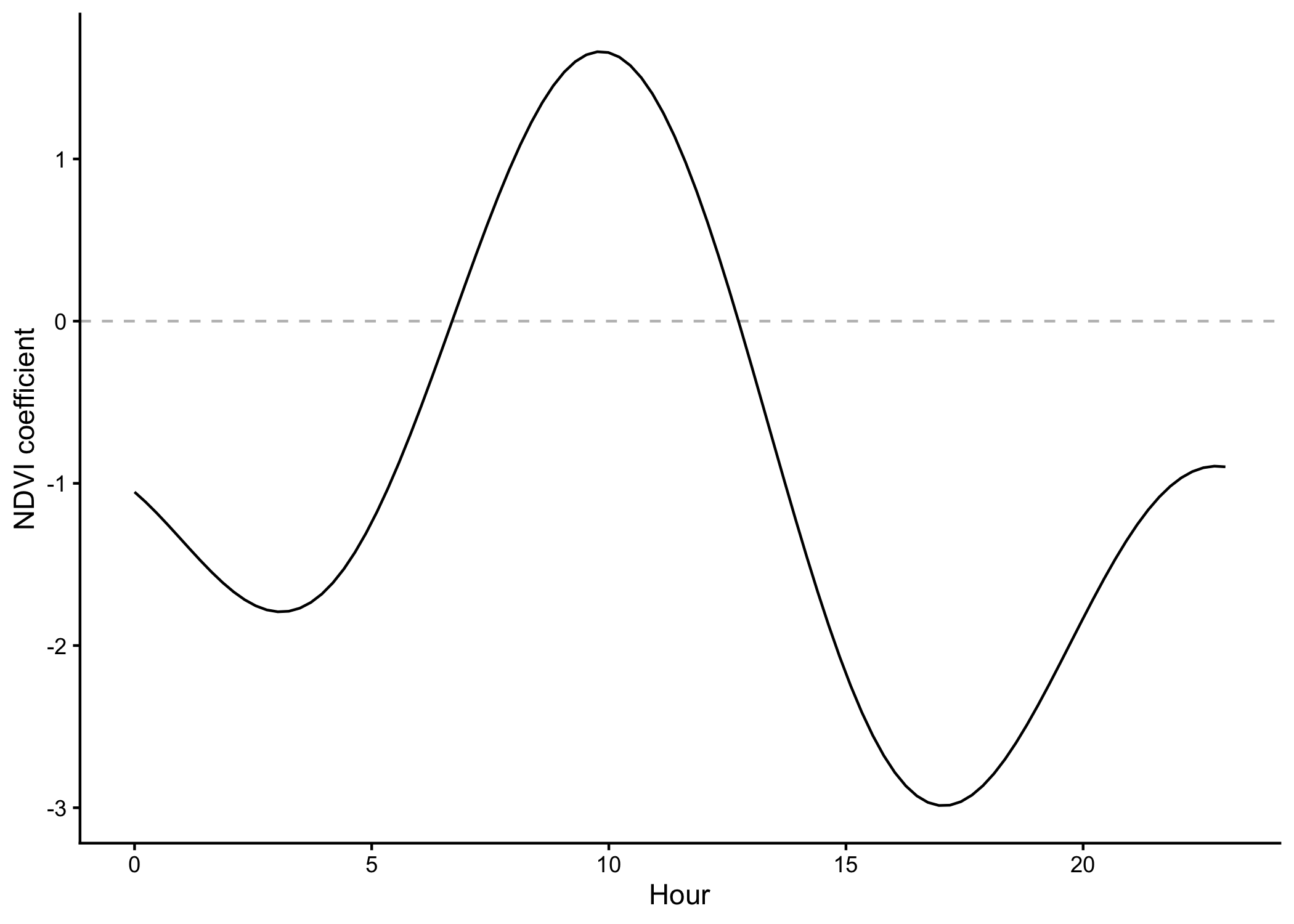

Calculate confidence intervals across time and plot

Code

sample_hour <- 9 # hour to plot with a vertical dashed line

# Coefficient names we need
coef_names <- c("ndvi",
                "ndvi:sin_1_hour","ndvi:cos_1_hour",
                "ndvi:sin_2_hour","ndvi:cos_2_hour")

# coefficients and V from the underlying clogit model
beta <- coef(ssf_harmonics$model)[coef_names]
V    <- vcov(ssf_harmonics$model)[coef_names, coef_names, drop = FALSE]

# Build design for each hour
ndvi_temporal_ci <- tibble(hour = seq(0, 23, length.out = 231)) %>%
  mutate(
    sin_1 = sin(2 * pi * hour / 24),
    cos_1 = cos(2 * pi * hour / 24),
    sin_2 = sin(4 * pi * hour / 24),
    cos_2 = cos(4 * pi * hour / 24)
  ) %>%
  rowwise() %>%
  mutate(
    x = list(c(1, sin_1, cos_1, sin_2, cos_2)),
    est = as.numeric(matrix(unlist(x), nrow = 1) %*% beta),
    se  = sqrt(as.numeric(matrix(unlist(x), nrow = 1) %*% V %*% matrix(unlist(x), ncol = 1))),
    lo  = est - 1.96 * se,
    hi  = est + 1.96 * se
  ) %>%
  ungroup() %>%
  select(hour, est, se, lo, hi)

# Plot with ribbon
ggplot(ndvi_temporal_ci, aes(x = hour)) +
  geom_hline(yintercept = 0, linetype = "dashed", colour = "black") +
  geom_vline(xintercept = 9, linetype = "dashed", colour = "orange") +
  geom_vline(xintercept = 17, linetype = "dashed", colour = "skyblue") +
  geom_ribbon(aes(ymin = lo, ymax = hi), alpha = 0.2) +
  geom_line(aes(y = est)) +
  labs(title = "harmonics(ndvi)", x = "Hour", y = expression(beta[NDVI]), fill = NULL) +
  scale_x_continuous(breaks = seq(0, 24, by = 4)) +
  scale_y_continuous(limits = c(-5,3.5), breaks = seq(-5, 4, by = 1)) +
  theme_classic()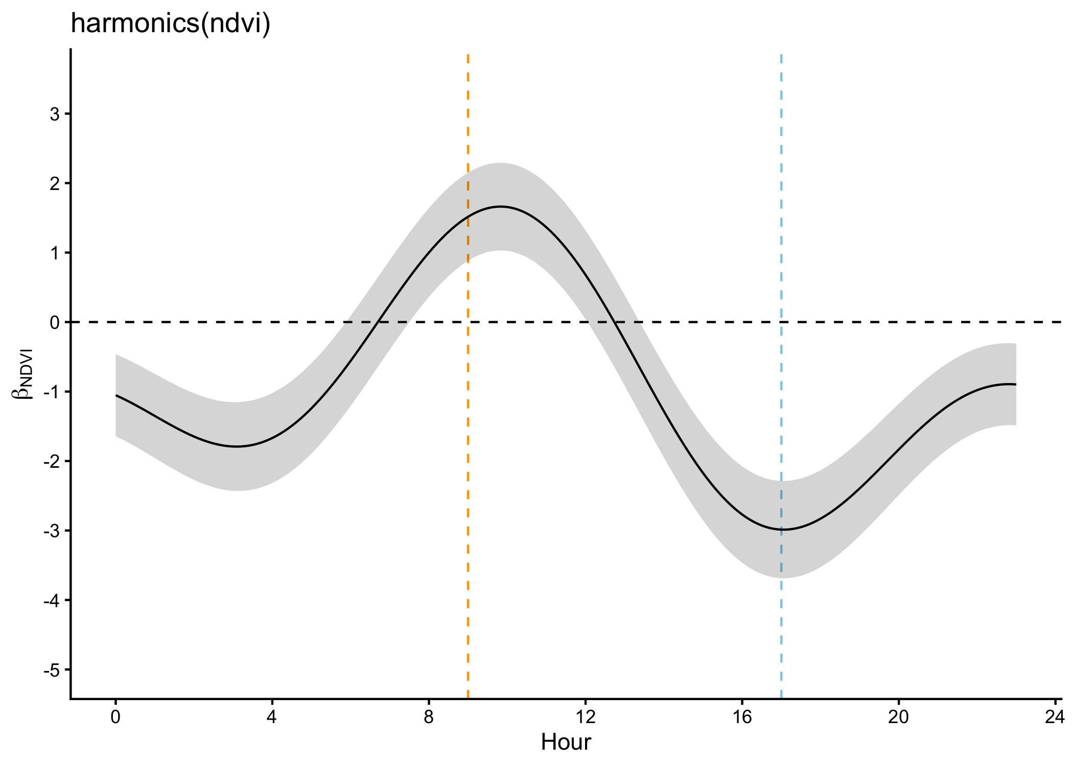

Code

ggsave(paste0(plot_save_path, "/ndvi_harmonic_coef_response_id", which_buffalo, ".png"),
       width = 150, height = 80, units = "mm", dpi = 600)

Pull out a response curve from one of the hours

Code

sample_hours <- c(9, 17)

ndvi_coef_df <- purrr::map_dfr(sample_hours, function(sample_hour) {
  
  # extract the NDVI coefficient and its standard error
  ndvi_coef <- ndvi_temporal_ci %>% filter(hour == sample_hour) %>% pull(est)
  ndvi_coef_se <- ndvi_temporal_ci %>% filter(hour == sample_hour) %>% pull(se)
  
  # calculate the RSS for each NDVI value
  data.frame(
    ndvi_values = ndvi_values,
    log_rss = ndvi_values * ndvi_coef,
    rss = exp(ndvi_values * ndvi_coef),
    se_prediction = abs(ndvi_values) * ndvi_coef_se
  ) %>% mutate(hour = as.factor(sample_hour), .before = ndvi_values)
})

# plot the response curve
ggplot(data = ndvi_coef_df) +
  geom_hline(yintercept = 1, linetype = "dashed", colour = "grey") +
  geom_ribbon(aes(x = ndvi_values, 
                  ymin = exp(log_rss - 1.96 * se_prediction), 
                  ymax = exp(log_rss + 1.96 * se_prediction),
                  fill = hour), 
              alpha = 0.5) +
  geom_line(aes(x = ndvi_values, y = rss, colour = hour), 
            linewidth = 1) +
  geom_rug(data = buffalo_ssf_data %>% filter(case_ == T), 
           aes(x = ndvi), alpha = 0.25, sides="b") +
  scale_colour_manual(values = c("orange", "skyblue")) +
  scale_fill_manual(values = c("orange", "skyblue")) +
  scale_x_continuous(breaks = seq(-0.2, 0.8, by = 0.1)) +
  scale_y_continuous(limits = c(0, 5.5)) +
  labs(x = "NDVI", y = "RSS") +
  theme_classic() +
  theme(legend.position = "none")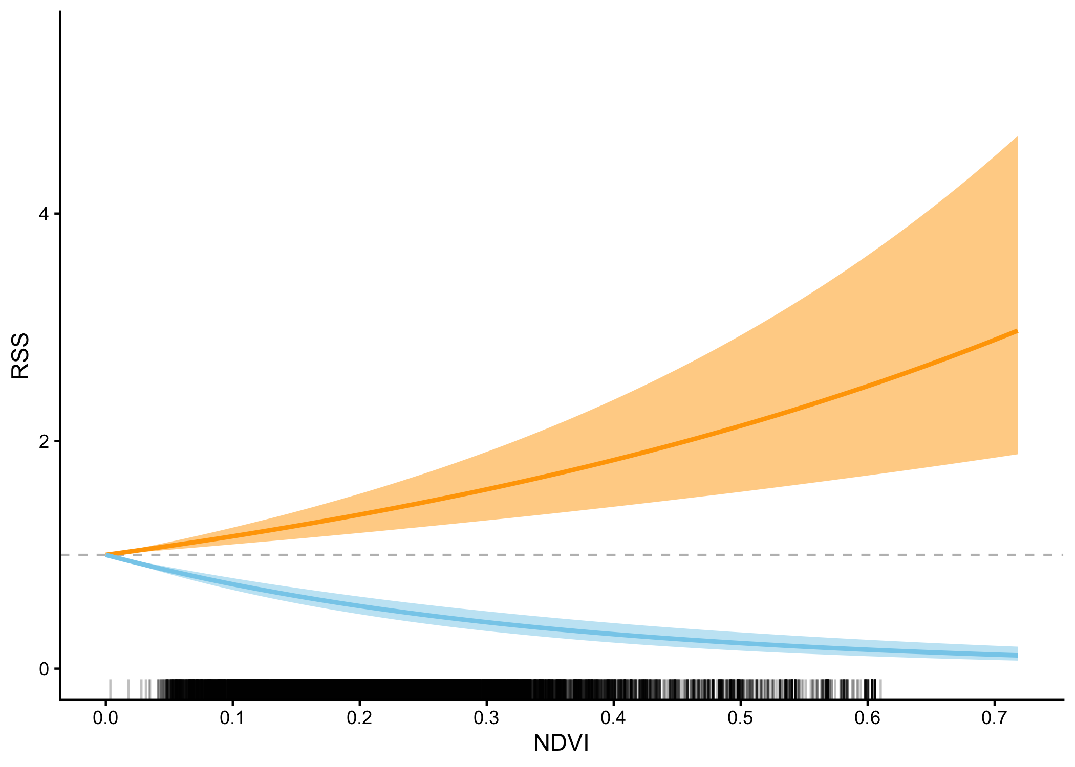

Code

ggsave(paste0(plot_save_path, "/ndvi_linear_response_sample_hour_id", which_buffalo, ".png"),
       width = 70, height = 80, units = "mm", dpi = 600)

Manually create the selection surface

Code

ndvi_harmonic_reconstruction <- function(ssf_harmonic_model, ndvi_value, hour) {
  
  ndvi_coef <- ssf_harmonic_model$model$coefficients["ndvi"]
  ndvi_sin_1_coef <- ssf_harmonic_model$model$coefficients["ndvi:sin_1_hour"]
  ndvi_cos_1_coef <- ssf_harmonic_model$model$coefficients["ndvi:cos_1_hour"]
  ndvi_sin_2_coef <- ssf_harmonic_model$model$coefficients["ndvi:sin_2_hour"]
  ndvi_cos_2_coef <- ssf_harmonic_model$model$coefficients["ndvi:cos_2_hour"]
  
  sin_1_hour <- sin(2 * pi * hour / 24)
  cos_1_hour <- cos(2 * pi * hour / 24)
  sin_2_hour <- sin(4 * pi * hour / 24)
  cos_2_hour <- cos(4 * pi * hour / 24)
  
  log_rss <- as.numeric(ndvi_value * ndvi_coef + 
                          ndvi_value * sin_1_hour * ndvi_sin_1_coef + 
                          ndvi_value * cos_1_hour * ndvi_cos_1_coef + 
                          ndvi_value * sin_2_hour * ndvi_sin_2_coef + 
                          ndvi_value * cos_2_hour * ndvi_cos_2_coef)
  
  return(log_rss)
  
}

# test function
ndvi_harmonic_reconstruction(ssf_harmonics, 
                             ndvi_values[1], 
                             hour = 12)

[1] 0

Create table of NDVI and hour values

Code

ndvi_hour_values <- expand.grid(ndvi = ndvi_values, 
                                hour = seq(0, 23, length.out = length(ndvi_values)))

ndvi_hour_values$ssf_linear_log_rss <- mapply(ndvi_harmonic_reconstruction, 
                                        ssf_harmonic_model = list(ssf_harmonics), 
                                        ndvi_value = ndvi_hour_values$ndvi, 
                                        hour = ndvi_hour_values$hour)

# plot the response curve
ggplot(data = ndvi_hour_values) +
  geom_point(aes(x = hour, y = ndvi, colour = ssf_linear_log_rss)) +
  labs(x = "Hour", y = "NDVI", colour = "log RSS") +
  scale_colour_viridis_c() +
  theme_classic()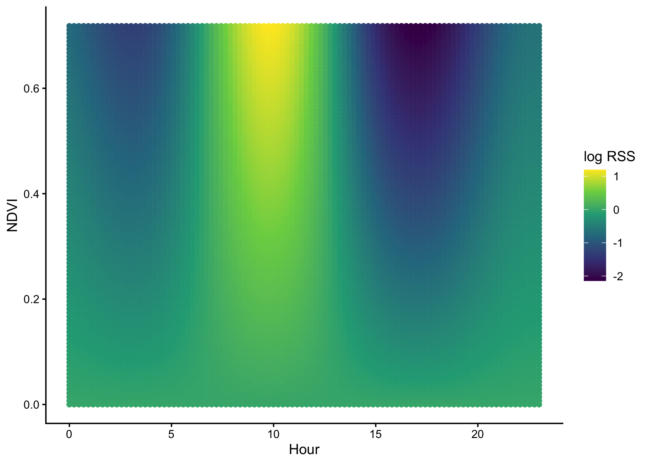

Code

max_abs_colour <- max(abs(range(ndvi_hour_values$ssf_linear_log_rss)))

# plot the selection surface
ggplot() +
  geom_raster(data = ndvi_hour_values,
       aes(x = hour, y = ndvi, fill = ssf_linear_log_rss)) +
  labs(title = "harmonics(ndvi)", x = "Hour", y = "NDVI", fill = "log-RSS") +
  geom_contour(data = ndvi_hour_values,
       aes(x = hour, y = ndvi, z = ssf_linear_log_rss), 
       colour = "black") +
  geom_contour(data = ndvi_hour_values,
       aes(x = hour, y = ndvi, z = ssf_linear_log_rss),
       breaks = 0, colour = "black", linetype = "solid", linewidth = 1) +
  scale_fill_distiller(palette = "RdBu", type = "div", direction = 1,
    limits = c(-max_abs_colour, max_abs_colour)) +   # symmetric around 0) 
  coord_cartesian(expand = FALSE) +
  geom_rug(data = buffalo_ssf_data %>% filter(case_ == T),
           aes(y = ndvi), alpha = 0.1, length = unit(0.015, "npc"), sides="l") +
  scale_y_continuous(breaks = seq(-0.2, 0.8, by = 0.1)) +
  theme_bw()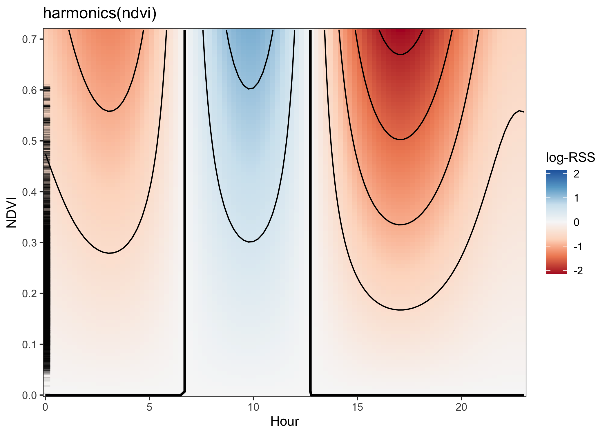

Code

ggsave(paste0(plot_save_path, "/ndvi_harmonic_response_id", which_buffalo, ".png"),
       width = 150, height = 80, units = "mm", dpi = 600)

Fit harmonic model with quadratic terms

Code

ssf_harmonics_quadratic <- amt::fit_issf(case_ ~ 
                                 
                                 # linear terms
                                 ndvi + 
                                 ndvi:sin_1_hour + ndvi:cos_1_hour +
                                 ndvi:sin_2_hour + ndvi:cos_2_hour +
                                 
                                 # quadratic terms
                                 ndvi_sq +
                                 ndvi_sq:sin_1_hour + ndvi_sq:cos_1_hour +
                                 ndvi_sq:sin_2_hour + ndvi_sq:cos_2_hour +
                                 
                                 sl_ + log_sl + cos_ta +
                                   
                                 strata(step_id_),
                               data = buffalo_ssf_data)

summary(ssf_harmonics_quadratic)

Call:
coxph(formula = Surv(rep(1, 106678L), case_) ~ ndvi + ndvi:sin_1_hour + 
    ndvi:cos_1_hour + ndvi:sin_2_hour + ndvi:cos_2_hour + ndvi_sq + 
    ndvi_sq:sin_1_hour + ndvi_sq:cos_1_hour + ndvi_sq:sin_2_hour + 
    ndvi_sq:cos_2_hour + sl_ + log_sl + cos_ta + strata(step_id_), 
    data = data, method = "exact")

  n= 106678, number of events= 9698 

                         coef  exp(coef)   se(coef)       z Pr(>|z|)    
ndvi                4.484e+00  8.860e+01  5.084e-01   8.819  < 2e-16 ***
ndvi_sq            -9.156e+00  1.056e-04  8.458e-01 -10.825  < 2e-16 ***
sl_                -1.736e-05  1.000e+00  3.212e-05  -0.540  0.58899    
log_sl              7.769e-03  1.008e+00  5.727e-03   1.357  0.17491    
cos_ta             -1.503e-02  9.851e-01  1.506e-02  -0.999  0.31803    
ndvi:sin_1_hour     6.955e-01  2.005e+00  7.242e-01   0.960  0.33687    
ndvi:cos_1_hour     1.014e+00  2.757e+00  7.054e-01   1.438  0.15051    
ndvi:sin_2_hour    -1.992e+00  1.364e-01  7.216e-01  -2.761  0.00577 ** 
ndvi:cos_2_hour     9.941e-01  2.702e+00  7.059e-01   1.408  0.15905    
ndvi_sq:sin_1_hour  7.542e-01  2.126e+00  1.234e+00   0.611  0.54102    
ndvi_sq:cos_1_hour -2.856e+00  5.750e-02  1.135e+00  -2.516  0.01188 *  
ndvi_sq:sin_2_hour  1.387e+00  4.004e+00  1.187e+00   1.169  0.24238    
ndvi_sq:cos_2_hour  1.546e-01  1.167e+00  1.180e+00   0.131  0.89575    
---
Signif. codes:  0 '***' 0.001 '**' 0.01 '*' 0.05 '.' 0.1 ' ' 1

                   exp(coef) exp(-coef) lower .95 upper .95
ndvi               8.860e+01  1.129e-02 3.271e+01 2.400e+02
ndvi_sq            1.055e-04  9.474e+03 2.011e-05 5.539e-04
sl_                1.000e+00  1.000e+00 9.999e-01 1.000e+00
log_sl             1.008e+00  9.923e-01 9.966e-01 1.019e+00
cos_ta             9.851e-01  1.015e+00 9.564e-01 1.015e+00
ndvi:sin_1_hour    2.005e+00  4.988e-01 4.849e-01 8.289e+00
ndvi:cos_1_hour    2.757e+00  3.627e-01 6.918e-01 1.099e+01
ndvi:sin_2_hour    1.364e-01  7.331e+00 3.316e-02 5.611e-01
ndvi:cos_2_hour    2.702e+00  3.701e-01 6.774e-01 1.078e+01
ndvi_sq:sin_1_hour 2.126e+00  4.704e-01 1.894e-01 2.387e+01
ndvi_sq:cos_1_hour 5.750e-02  1.739e+01 6.214e-03 5.322e-01
ndvi_sq:sin_2_hour 4.004e+00  2.498e-01 3.912e-01 4.098e+01
ndvi_sq:cos_2_hour 1.167e+00  8.568e-01 1.156e-01 1.178e+01

Concordance= 0.546  (se = 0.004 )
Likelihood ratio test= 267.6  on 13 df,   p=<2e-16
Wald test            = 217.7  on 13 df,   p=<2e-16
Score (logrank) test = 218.6  on 13 df,   p=<2e-16

Code

AIC(ssf_harmonics_quadratic)

[1] 46267.92

Manually create the selection surface

Code

ndvi_harmonic_reconstruction <- function(ssf_harmonic_model, ndvi_value, hour) {
  
  # linear terms
  ndvi_coef <- ssf_harmonic_model$model$coefficients["ndvi"]
  ndvi_sin_1_coef <- ssf_harmonic_model$model$coefficients["ndvi:sin_1_hour"]
  ndvi_cos_1_coef <- ssf_harmonic_model$model$coefficients["ndvi:cos_1_hour"]
  ndvi_sin_2_coef <- ssf_harmonic_model$model$coefficients["ndvi:sin_2_hour"]
  ndvi_cos_2_coef <- ssf_harmonic_model$model$coefficients["ndvi:cos_2_hour"]
  
  # quadratic terms
  ndvi_sq_coef <- ssf_harmonic_model$model$coefficients["ndvi_sq"]
  ndvi_sq_sin_1_coef <- ssf_harmonic_model$model$coefficients["ndvi_sq:sin_1_hour"]
  ndvi_sq_cos_1_coef <- ssf_harmonic_model$model$coefficients["ndvi_sq:cos_1_hour"]
  ndvi_sq_sin_2_coef <- ssf_harmonic_model$model$coefficients["ndvi_sq:sin_2_hour"]
  ndvi_sq_cos_2_coef <- ssf_harmonic_model$model$coefficients["ndvi_sq:cos_2_hour"]
  
  sin_1_hour <- sin(2 * pi * hour / 24)
  cos_1_hour <- cos(2 * pi * hour / 24)
  sin_2_hour <- sin(4 * pi * hour / 24)
  cos_2_hour <- cos(4 * pi * hour / 24)
  
  linear_part <- ndvi_value * ndvi_coef + 
    ndvi_value * sin_1_hour * ndvi_sin_1_coef + 
    ndvi_value * cos_1_hour * ndvi_cos_1_coef + 
    ndvi_value * sin_2_hour * ndvi_sin_2_coef + 
    ndvi_value * cos_2_hour * ndvi_cos_2_coef
  
  ndvi_sq_value <- ndvi_value^2
  
  quadratic_part <- ndvi_sq_value * ndvi_sq_coef + 
    ndvi_sq_value * sin_1_hour * ndvi_sq_sin_1_coef + 
    ndvi_sq_value * cos_1_hour * ndvi_sq_cos_1_coef + 
    ndvi_sq_value * sin_2_hour * ndvi_sq_sin_2_coef + 
    ndvi_sq_value * cos_2_hour * ndvi_sq_cos_2_coef
  
  return(as.numeric(linear_part + quadratic_part))
  
}

# test function
ndvi_harmonic_reconstruction(ssf_harmonics_quadratic, ndvi_values[1], hour = 12)

[1] 0

Create table of NDVI and hour values

Code

ndvi_hour_values <- expand.grid(ndvi = ndvi_values, 
                                hour = seq(0, 23, length.out = length(ndvi_values)))

ndvi_hour_values$ssf_quadratic_log_rss <- mapply(ndvi_harmonic_reconstruction, 
                                                 ssf_harmonic_model = list(ssf_harmonics_quadratic), 
                                                 ndvi_value = ndvi_hour_values$ndvi, 
                                                 hour = ndvi_hour_values$hour)

# plot the response curve
ggplot(data = ndvi_hour_values) +
  geom_point(aes(x = hour, y = ndvi, colour = ssf_quadratic_log_rss)) +
  labs(x = "Hour", y = "NDVI", colour = "log RSS") +
  scale_colour_viridis_c() +
  scale_y_continuous(breaks = seq(-0.2, 0.8, by = 0.1)) +
  theme_classic()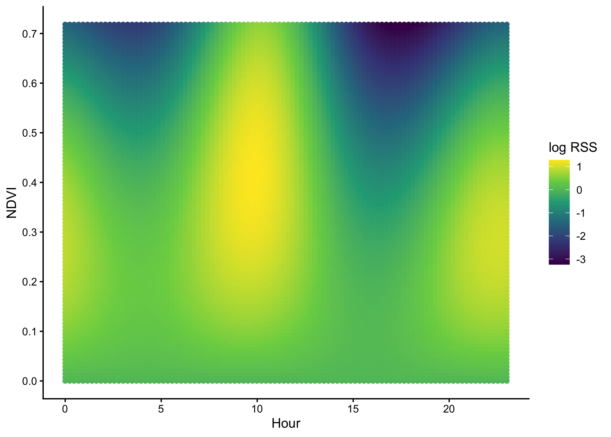

Code

max_abs_colour <- max(abs(range(ndvi_hour_values$ssf_quadratic_log_rss)))

# plot the selection surface
ggplot() +
  geom_raster(data = ndvi_hour_values,
       aes(x = hour, y = ndvi, fill = ssf_quadratic_log_rss)) +
  labs(title = "harmonics(ndvi + ndvi^2)", x = "Hour", y = "NDVI", fill = "log-RSS") +
  geom_contour(data = ndvi_hour_values,
       aes(x = hour, y = ndvi, z = ssf_quadratic_log_rss), 
       colour = "black") +
  geom_contour(data = ndvi_hour_values,
       aes(x = hour, y = ndvi, z = ssf_quadratic_log_rss),
       breaks = 0, colour = "black", linetype = "solid", linewidth = 1) +
  geom_vline(xintercept = 9, linetype = "dashed", colour = "orange") +
  geom_vline(xintercept = 17, linetype = "dashed", colour = "skyblue") +
  scale_fill_distiller(palette = "RdBu", type = "div", direction = 1,
                       limits = c(-max_abs_colour, max_abs_colour)) +
  coord_cartesian(expand = FALSE) +
  geom_rug(data = buffalo_ssf_data %>% filter(case_ == T),
           aes(y = ndvi), alpha = 0.25, length = unit(0.015, "npc"), sides="l") +
  scale_y_continuous(breaks = seq(-0.2, 0.8, by = 0.1)) +
  theme_bw()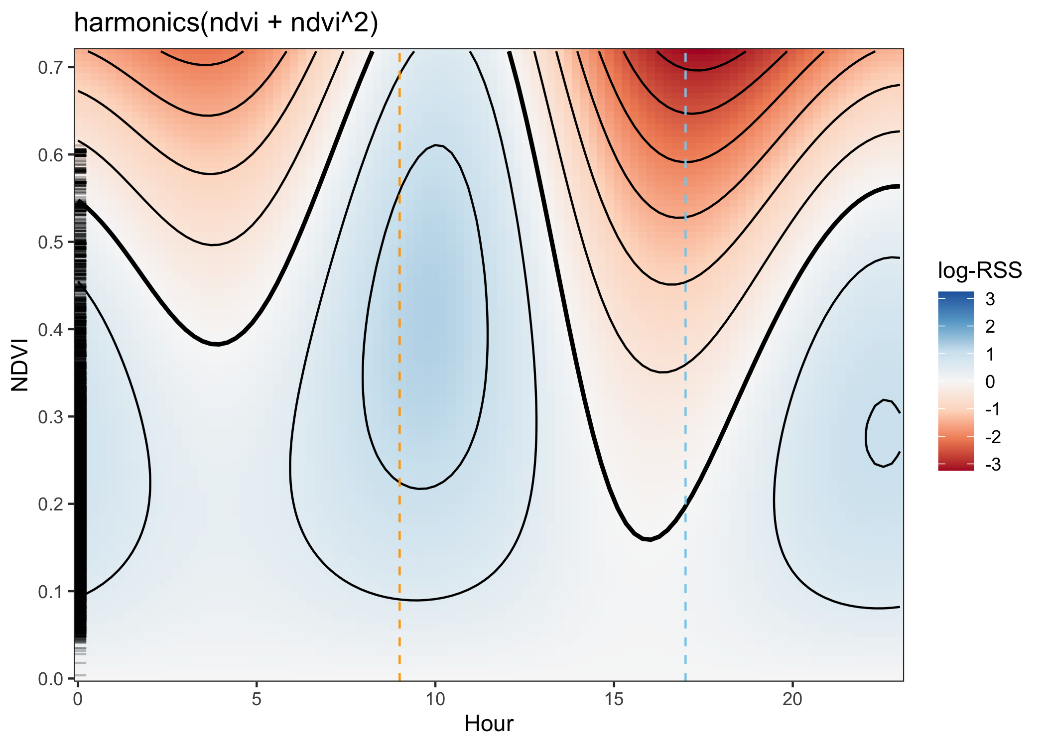

Code

ggsave(paste0(plot_save_path, "/ndvi_harmonic_quadratic_response_id", which_buffalo, ".png"),
       width = 150, height = 80, units = "mm", dpi = 600)

Pull out a response curve from one of the hours

Code

sample_hours <- c(9, 17)

curve_df <- purrr::map_dfr(sample_hours, function(sample_hour) {
  
  # Harmonics at sample hour
  s1 <- sin(2 * pi * sample_hour / 24)
  c1 <- cos(2 * pi * sample_hour / 24)
  s2 <- sin(4 * pi * sample_hour / 24)
  c2 <- cos(4 * pi * sample_hour / 24)
  
  mod   <- ssf_harmonics_quadratic$model
  betas <- coef(mod)
  V     <- vcov(mod)
  cn    <- names(betas)
  
  # For each NDVI value, build the contrast vector g such that g'β = log-RSS
  purrr::map_dfr(ndvi_values, function(x) {
    
    g <- setNames(numeric(length(betas)), cn)
    
    # linear term: x * (β_ndvi + harmonics)
    g["ndvi"]            <- x
    g["ndvi:sin_1_hour"] <- x * s1
    g["ndvi:cos_1_hour"] <- x * c1
    g["ndvi:sin_2_hour"] <- x * s2
    g["ndvi:cos_2_hour"] <- x * c2
    
    # quadratic term: x² * (β_ndvi_sq + harmonics)
    g["ndvi_sq"]             <- x^2
    g["ndvi_sq:sin_1_hour"]  <- x^2 * s1
    g["ndvi_sq:cos_1_hour"]  <- x^2 * c1
    g["ndvi_sq:sin_2_hour"]  <- x^2 * s2
    g["ndvi_sq:cos_2_hour"]  <- x^2 * c2
    
    log_rss <- as.numeric(g %*% betas)
    se_log  <- sqrt(as.numeric(t(g) %*% V %*% g))
    
    data.frame(
      hour    = sample_hour,
      ndvi    = x,
      log_rss = log_rss,
      rss     = exp(log_rss),
      # delta method on the RSS scale: SE_rss ≈ exp(log_rss) * SE_log
      rss_lwr = exp(log_rss - 1.96 * se_log),
      rss_upr = exp(log_rss + 1.96 * se_log)
    )
  })
})


# plot the response curve
ggplot(curve_df, aes(x = ndvi)) +
  geom_hline(yintercept = 1, linetype = "dashed", colour = "grey") +
  geom_ribbon(aes(ymin = rss_lwr, ymax = rss_upr, fill = as.factor(hour)), 
              alpha = 0.5) +
  geom_line(aes(y = rss, colour = as.factor(hour)), linewidth = 1) +
  geom_rug(data = buffalo_ssf_data %>% filter(case_ == T), 
           aes(x = ndvi), alpha = 0.25, sides="b") +
  scale_colour_manual(values = c("orange", "skyblue")) +
  scale_fill_manual(values = c("orange", "skyblue")) +
  scale_x_continuous(breaks = seq(-0.2, 0.8, by = 0.1)) + 
  scale_y_continuous(limits = c(0, 5.5)) +
  labs(x = "NDVI", y = "RSS") +
  theme_classic() +
  theme(legend.position = "none")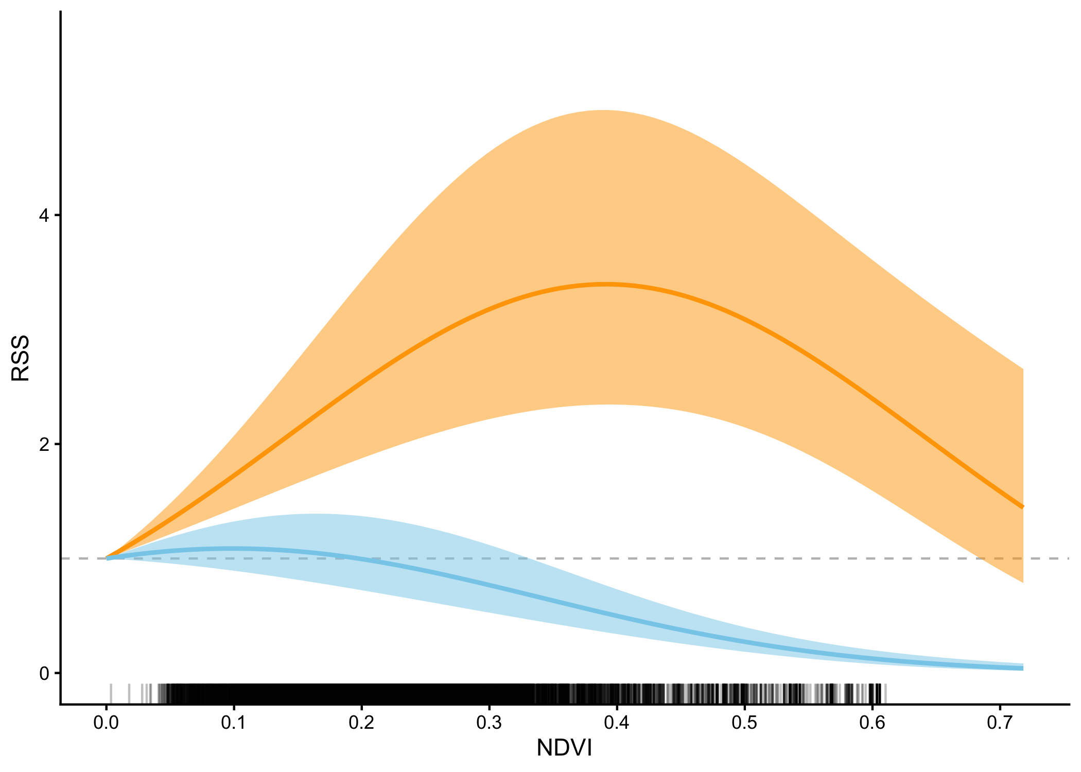

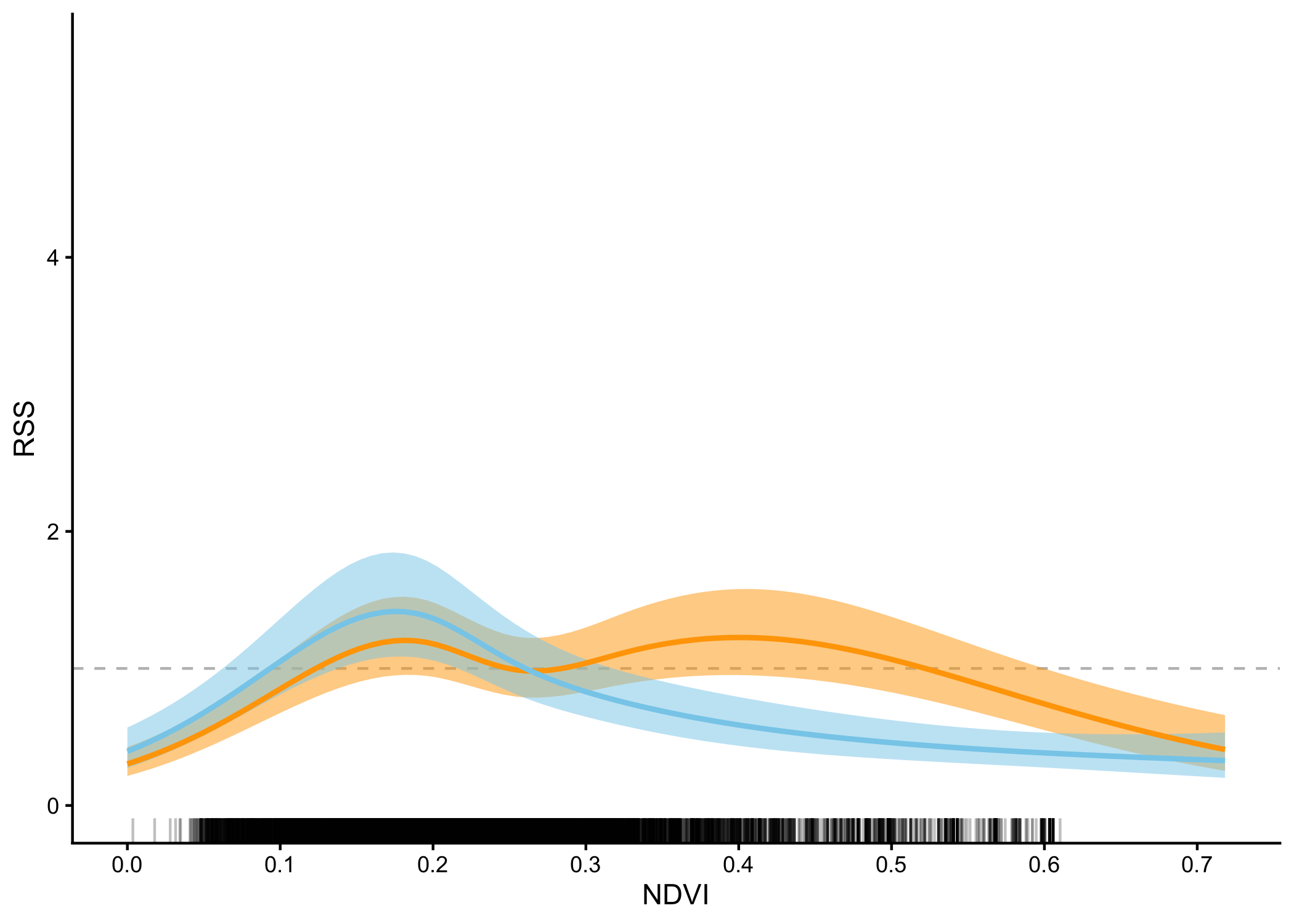
Code

ggsave(paste0(plot_save_path, "/ndvi_quadratic_response_sample_hour_id", which_buffalo, ".png"),
       width = 70, height = 80, units = "mm", dpi = 600)

Temporal dynamics with smooth terms

Code

# fit an ssf gam model
# We set the knots explicitly at 0 and 24. Without this, mgcv places the cyclic
# endpoints at the range of the data (0 and 23), which wraps hour 23 onto hour 0
# and squeezes an hour out of the daily cycle.
ssf_gam_temporal <- mgcv::gam(cbind(times, step_id_) ~
                       s(hour, by = ndvi, bs = "cc") + #, k = 5
                       sl_ + log_sl + cos_ta,
                     knots = list(hour = c(0, 24)),
                     data = buffalo_ssf_data,
                     family = cox.ph,
                     weight = case_)

summary(ssf_gam_temporal)


Family: Cox PH 
Link function: identity 

Formula:
cbind(times, step_id_) ~ s(hour, by = ndvi, bs = "cc") + sl_ + 
    log_sl + cos_ta

Parametric coefficients:
         Estimate Std. Error z value Pr(>|z|)
sl_    -1.933e-06  3.209e-05  -0.060    0.952
log_sl  3.548e-03  5.697e-03   0.623    0.533
cos_ta -1.385e-02  1.505e-02  -0.920    0.358

Approximate significance of smooth terms:
               edf Ref.df Chi.sq p-value    
s(hour):ndvi 8.104   8.78  149.1  <2e-16 ***
---
Signif. codes:  0 '***' 0.001 '**' 0.01 '*' 0.05 '.' 0.1 ' ' 1

Deviance explained = -3.48%
-REML =  23205  Scale est. = 1         n = 106678

Code

AIC(ssf_gam_temporal)

[1] 46363.75

Code

gam_smooths <- smooth_estimates(ssf_gam_temporal)

Code

gratia::draw(ssf_gam_temporal, rug = FALSE) +
  geom_hline(yintercept = 0, linetype = "dashed", colour = "grey60") +
  geom_vline(xintercept = 9, linetype = "dashed", colour = "orange") +
  geom_vline(xintercept = 17, linetype = "dashed", colour = "skyblue") +
  labs() +
  scale_x_continuous(breaks = seq(0, 24, by = 4)) +
  scale_y_continuous(limits = c(-5,3.5), breaks = seq(-5, 4, by = 1)) +
  labs(title = "s(hour, by = ndvi)",
       subtitle = NULL,
       caption = NULL,
       x = "Hour", 
       y = expression(beta[NDVI]), fill = NULL) +
  theme_classic()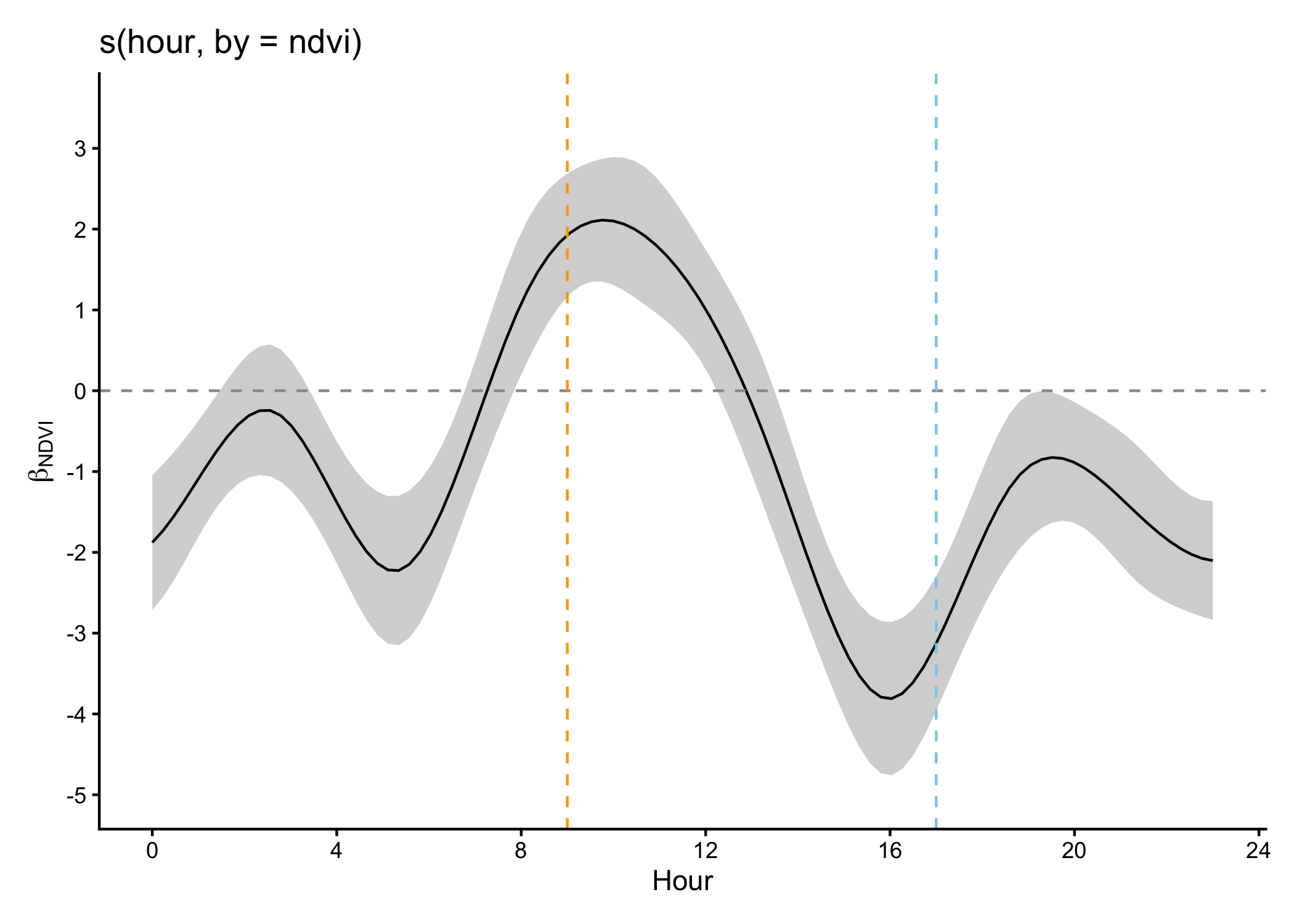

Code

ggsave(paste0(plot_save_path, "/ndvi_gam_coef_response_id", which_buffalo, ".png"),
       width = 150, height = 80, units = "mm", dpi = 600)

Pull out a response curve from one of the hours

Code

pred_data_hour9 <- pred_data
pred_data_hour9$hour <- 9

pred_data_hour17 <- pred_data
pred_data_hour17$hour <- 17

pred_data_hour9_17 <- bind_rows(pred_data_hour9, pred_data_hour17)

# Get predictions on log-scale with standard errors
predictions <- predict(ssf_gam_temporal, 
                      newdata = pred_data_hour9_17, 
                      type = "link",  # log-scale
                      se.fit = TRUE)

pred_data_hour9_17 <- pred_data_hour9_17 %>% 
  mutate(
    # Extract log RSS and standard errors
    log_rss = predictions$fit,
    se_log_rss = predictions$se.fit,
    # Calculate confidence intervals on log-scale
    log_rss_lower = log_rss - 1.96 * se_log_rss,
    log_rss_upper = log_rss + 1.96 * se_log_rss,
    # Transform to RSS scale
    rss = exp(log_rss),
    rss_lower = exp(log_rss_lower),
    rss_upper = exp(log_rss_upper)
  )

# plot the response curve
ggplot(data = pred_data_hour9_17) +
  geom_hline(yintercept = 1, linetype = "dashed", colour = "grey") +
  geom_ribbon(aes(x = ndvi, 
                  ymin = rss_lower, ymax = rss_upper,
                  fill = as.factor(hour)), 
              alpha = 0.5) +
  geom_line(aes(x = ndvi, y = rss, colour = as.factor(hour)), 
            linewidth = 1) +
  geom_rug(data = buffalo_ssf_data %>% filter(case_ == T), 
           aes(x = ndvi), alpha = 0.25, sides="b") +
  scale_colour_manual(values = c("orange", "skyblue")) +
  scale_fill_manual(values = c("orange", "skyblue")) +
  scale_x_continuous(breaks = seq(-0.2, 0.8, by = 0.1)) +
  scale_y_continuous(limits = c(0, 5.5)) +
  labs(x = "NDVI", y = "RSS") +
  theme_classic() +
  theme(legend.position = "none")

Warning: Removed 12 rows containing missing values or values outside the scale range
(`geom_ribbon()`).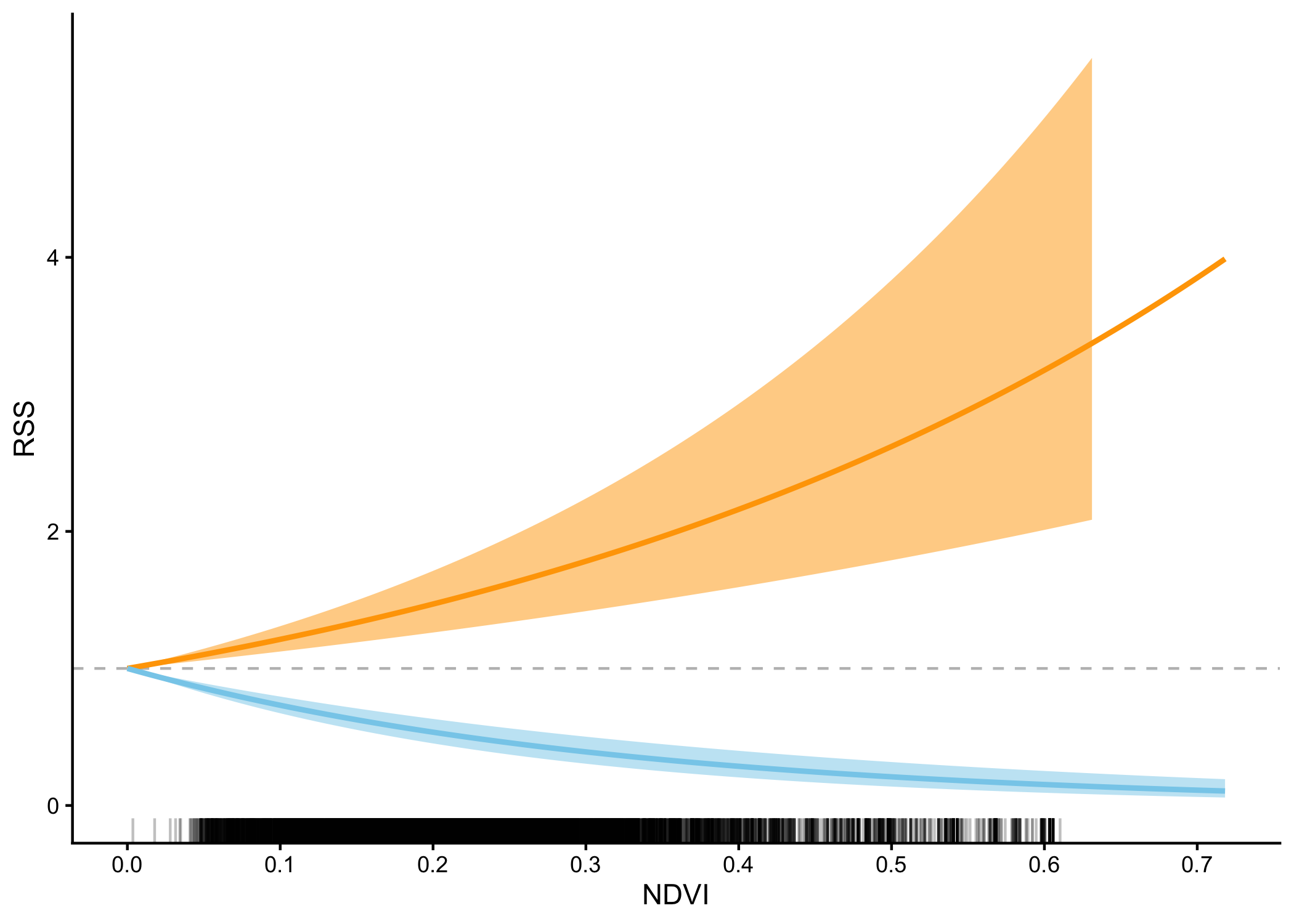

Code

ggsave(paste0(plot_save_path, "/ndvi_gam_response_sample_hour_id", which_buffalo, ".png"),
       width = 70, height = 80, units = "mm", dpi = 600)

Warning: Removed 12 rows containing missing values or values outside the scale range
(`geom_ribbon()`).

GAM selection surface

Code

ndvi_hour_values <- expand.grid(ndvi = ndvi_values, 
                                hour = seq(0, 23, length.out = length(ndvi_values)))

ndvi_hour_values <- ndvi_hour_values %>% mutate(
  sl_ = 0,
  log_sl = 0,
  cos_ta = 0
)

ndvi_hour_values

Code

# Get predictions on log-scale with standard errors
predictions <- predict(ssf_gam_temporal, 
                      newdata = ndvi_hour_values, 
                      type = "link",  # log-scale
                      se.fit = TRUE)

# Extract log RSS and standard errors
gam_log_rss <- predictions$fit
gam_se_log_rss <- predictions$se.fit

# Calculate confidence intervals on log-scale
gam_log_rss_lower <- gam_log_rss - 1.96 * gam_se_log_rss
gam_log_rss_upper <- gam_log_rss + 1.96 * gam_se_log_rss

# Transform to RSS scale
rss <- exp(gam_log_rss)
rss_lower <- exp(gam_log_rss_lower)
rss_upper <- exp(gam_log_rss_upper)

ndvi_hour_values <- ndvi_hour_values %>% mutate(
  gam_log_rss = gam_log_rss,
  gam_rss = exp(gam_log_rss),
  gam_log_rss_lower = as.numeric(gam_log_rss_lower),
  gam_log_rss_upper = as.numeric(gam_log_rss_upper)
)

max_abs_colour <- max(abs(range(ndvi_hour_values$gam_log_rss)))

# plot the selection surface
ggplot() +
  geom_raster(data = ndvi_hour_values,
       aes(x = hour, y = ndvi, fill = gam_log_rss)) +
  labs(title = "s(hour, by = ndvi)", x = "Hour", y = "NDVI", fill = "log-RSS") +
  geom_contour(data = ndvi_hour_values,
       aes(x = hour, y = ndvi, z = gam_log_rss), colour = "black") +
  scale_fill_distiller(palette = "RdBu", type = "div", direction = 1,
                       limits = c(-max_abs_colour, max_abs_colour)) +
  coord_cartesian(expand = FALSE) +
  geom_rug(data = buffalo_ssf_data %>% filter(case_ == T),
           aes(y = ndvi), alpha = 0.25, length = unit(0.015, "npc"), sides="l") +
  scale_y_continuous(breaks = seq(-0.2, 0.8, by = 0.1)) +
  theme_bw()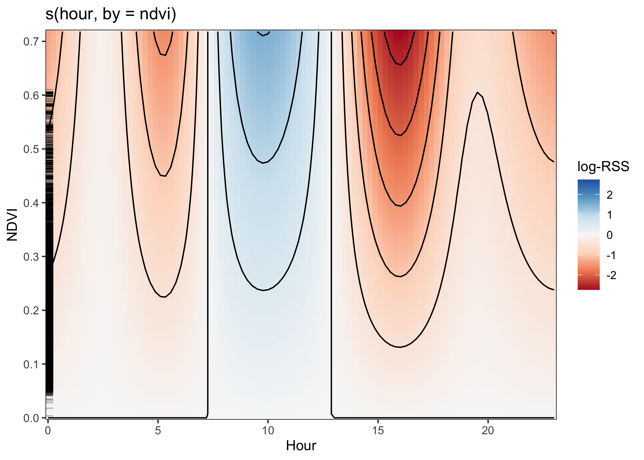

Code

ggsave(paste0(plot_save_path, "/ndvi_linear_gam_response_id", which_buffalo, ".png"),
       width = 150, height = 80, units = "mm", dpi = 600)

Fit 2D GAM smooth

Code

# fit an ssf gam model
# As above, set the cyclic knots for the hour margin explicitly at 0 and 24
ssf_gam2d_temporal2 <- mgcv::gam(cbind(times, step_id_) ~
                                  te(hour, ndvi, bs = c("cc", "cr")) + #, k = c(5, 5)
                       sl_ + log_sl + cos_ta,
                     knots = list(hour = c(0, 24)),
                     data = buffalo_ssf_data,
                     family = cox.ph,
                     weight = case_)

summary(ssf_gam2d_temporal2)


Family: Cox PH 
Link function: identity 

Formula:
cbind(times, step_id_) ~ te(hour, ndvi, bs = c("cc", "cr")) + 
    sl_ + log_sl + cos_ta

Parametric coefficients:
         Estimate Std. Error z value Pr(>|z|)  
sl_    -1.353e-05  3.207e-05  -0.422   0.6730  
log_sl  1.096e-02  5.751e-03   1.907   0.0566 .
cos_ta -1.299e-02  1.506e-02  -0.862   0.3886  
---
Signif. codes:  0 '***' 0.001 '**' 0.01 '*' 0.05 '.' 0.1 ' ' 1

Approximate significance of smooth terms:
                edf Ref.df Chi.sq p-value    
te(hour,ndvi) 11.72  13.37    351  <2e-16 ***
---
Signif. codes:  0 '***' 0.001 '**' 0.01 '*' 0.05 '.' 0.1 ' ' 1

Deviance explained = -0.0651%
-REML =  23099  Scale est. = 1         n = 106678

Code

AIC(ssf_gam2d_temporal2)

[1] 46149.4

Plot the smooth selection surface

Code

gratia::draw(ssf_gam2d_temporal2, rug = FALSE)

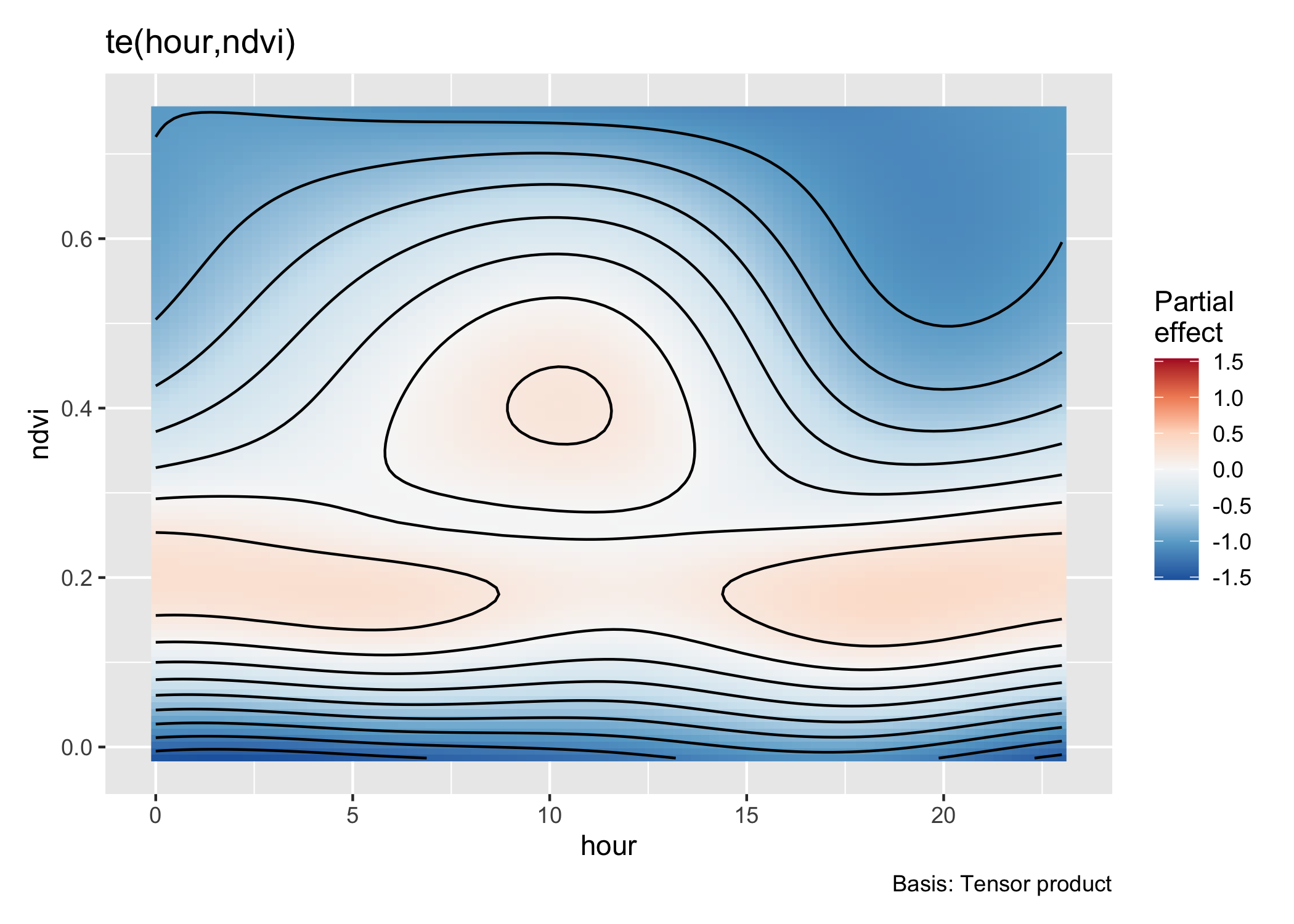
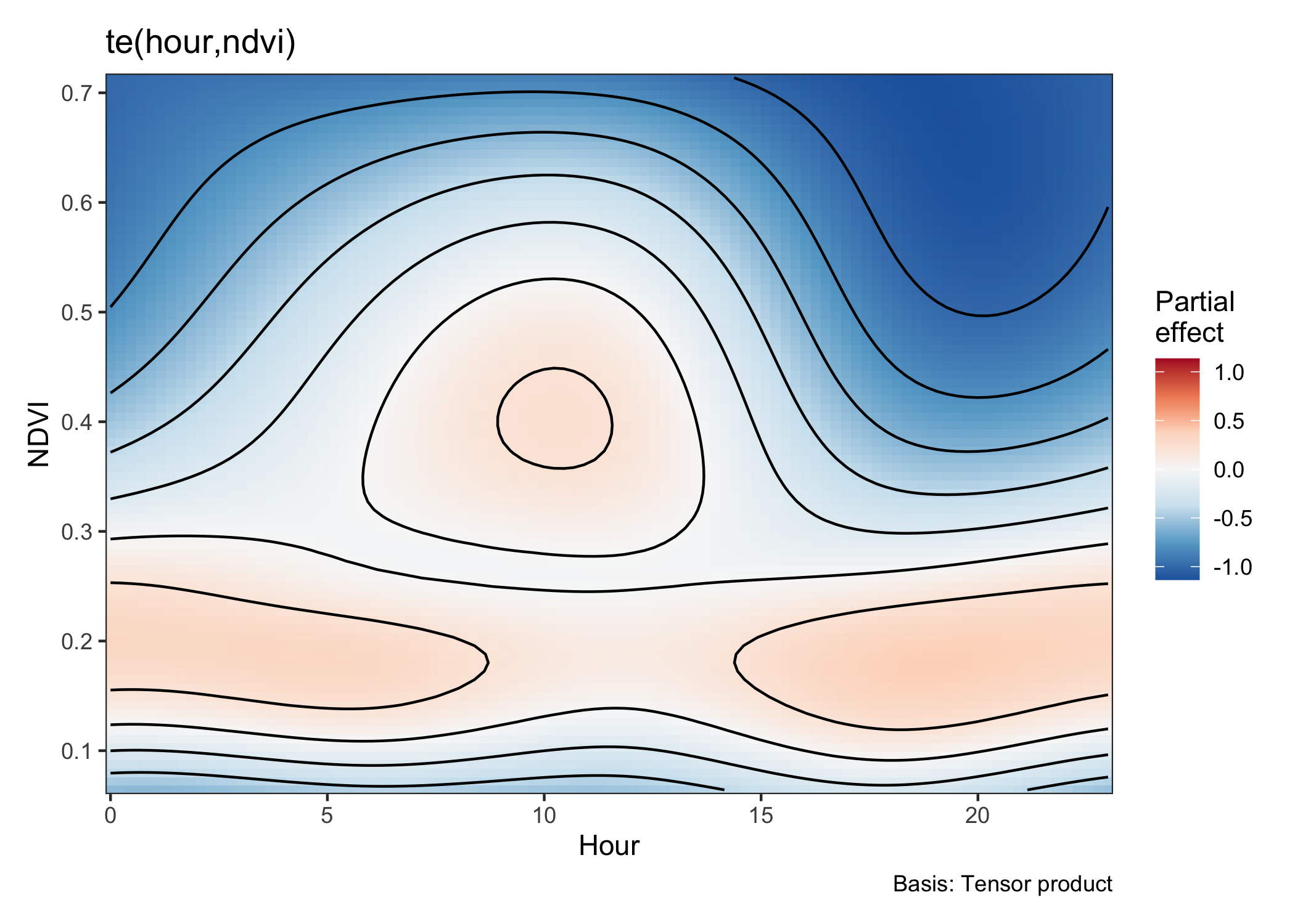
Code

gam_smooths <- smooth_estimates(ssf_gam2d_temporal2)
filtered_gam_smooths <- gam_smooths %>% filter(ndvi > ndvi_quantiles[1] & ndvi < ndvi_quantiles[2])

gratia::draw(filtered_gam_smooths) +
  coord_cartesian(expand = FALSE) +
  scale_y_continuous(breaks = seq(-0.2, 0.8, by = 0.1)) +
  labs(x = "Hour", y = "NDVI") +
  theme_bw()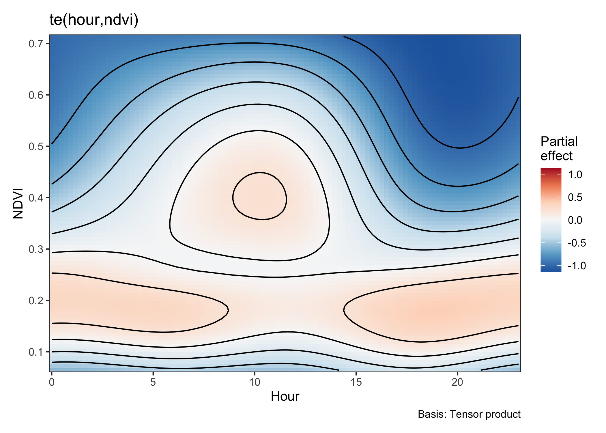

Code

ndvi_hour_values <- expand.grid(ndvi = ndvi_values, 
                                hour = seq(0, 23, length.out = length(ndvi_values)))

ndvi_hour_values <- ndvi_hour_values %>% mutate(
  sl_ = 0,
  log_sl = 0,
  cos_ta = 0
)

predictions <- predict(ssf_gam2d_temporal2, 
                      newdata = ndvi_hour_values, 
                      type = "link",  # log-scale
                      se.fit = TRUE)

# Extract log RSS and standard errors
gam_log_rss <- predictions$fit
gam_se_log_rss <- predictions$se.fit

# Calculate confidence intervals on log-scale
gam_log_rss_lower <- gam_log_rss - 1.96 * gam_se_log_rss
gam_log_rss_upper <- gam_log_rss + 1.96 * gam_se_log_rss

ndvi_hour_values <- ndvi_hour_values %>% mutate(
  gam_log_rss = gam_log_rss,
  gam_rss = exp(gam_log_rss),
  gam_log_rss_lower = as.numeric(gam_log_rss_lower),
  gam_log_rss_upper = as.numeric(gam_log_rss_upper)
)

# plot the selection surface
ggplot(data = ndvi_hour_values) +
  geom_point(aes(x = hour, y = ndvi, colour = gam_log_rss)) +
  labs(x = "Hour", y = "NDVI", colour = "log RSS") +
  scale_colour_viridis_c() +
  scale_y_continuous(breaks = seq(-0.2, 0.8, by = 0.1)) +
  theme_classic()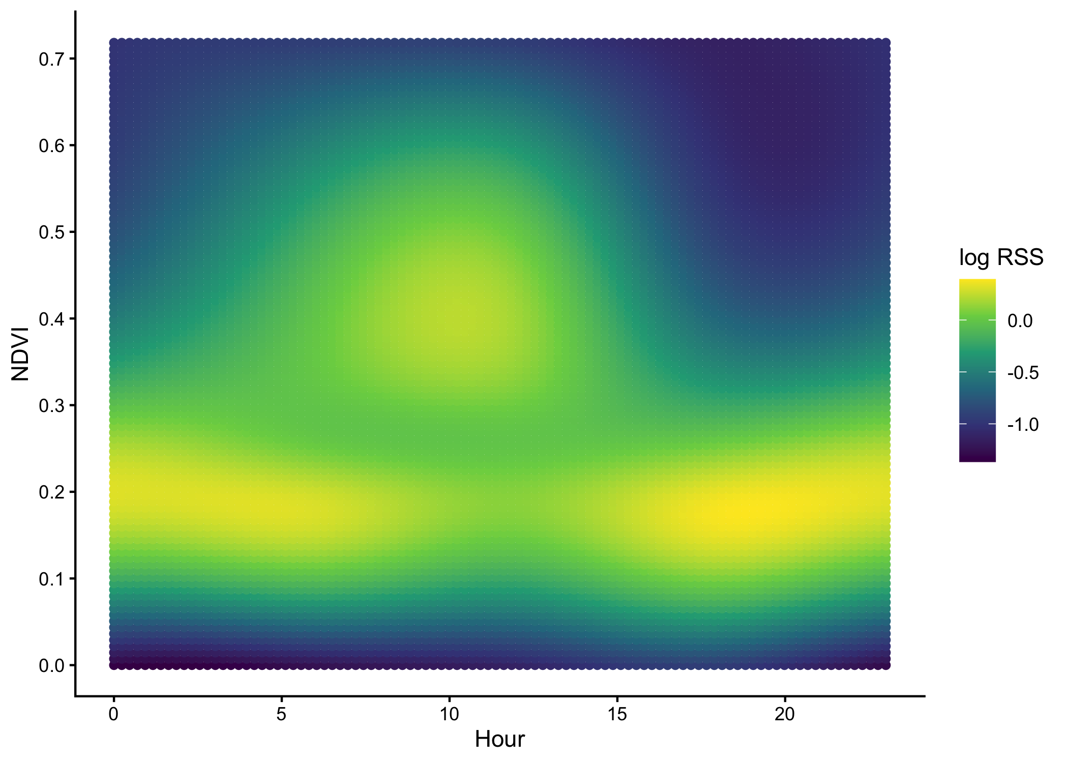

Code

gratia::draw(filtered_gam_smooths) +
  coord_cartesian(expand = FALSE) +
  scale_y_continuous(breaks = seq(-0.2, 0.8, by = 0.1)) +
  labs(x = "Hour", y = "NDVI") +
  theme_bw()

Code

max_abs_colour <- max(abs(range(ndvi_hour_values$gam_log_rss)))

# plot the selection surface
ggplot() +
  geom_raster(data = ndvi_hour_values,
       aes(x = hour, y = ndvi, fill = gam_log_rss)) +
  labs(title = "te(hour, ndvi)", x = "Hour", y = "NDVI", fill = "log-RSS") +
  geom_contour(data = ndvi_hour_values,
       aes(x = hour, y = ndvi, z = gam_log_rss), colour = "black") +
  geom_vline(xintercept = 9, linetype = "dashed", colour = "orange") +
  geom_vline(xintercept = 17, linetype = "dashed", colour = "skyblue") +
  scale_fill_distiller(palette = "RdBu", type = "div", direction = 1,
                       limits = c(-max_abs_colour, max_abs_colour)) +
  coord_cartesian(expand = FALSE) +
  geom_rug(data = buffalo_ssf_data %>% filter(case_ == T),
           aes(y = ndvi), alpha = 0.25, length = unit(0.015, "npc"), sides="l") +
  scale_y_continuous(breaks = seq(-0.2, 0.8, by = 0.1)) +
  theme_bw()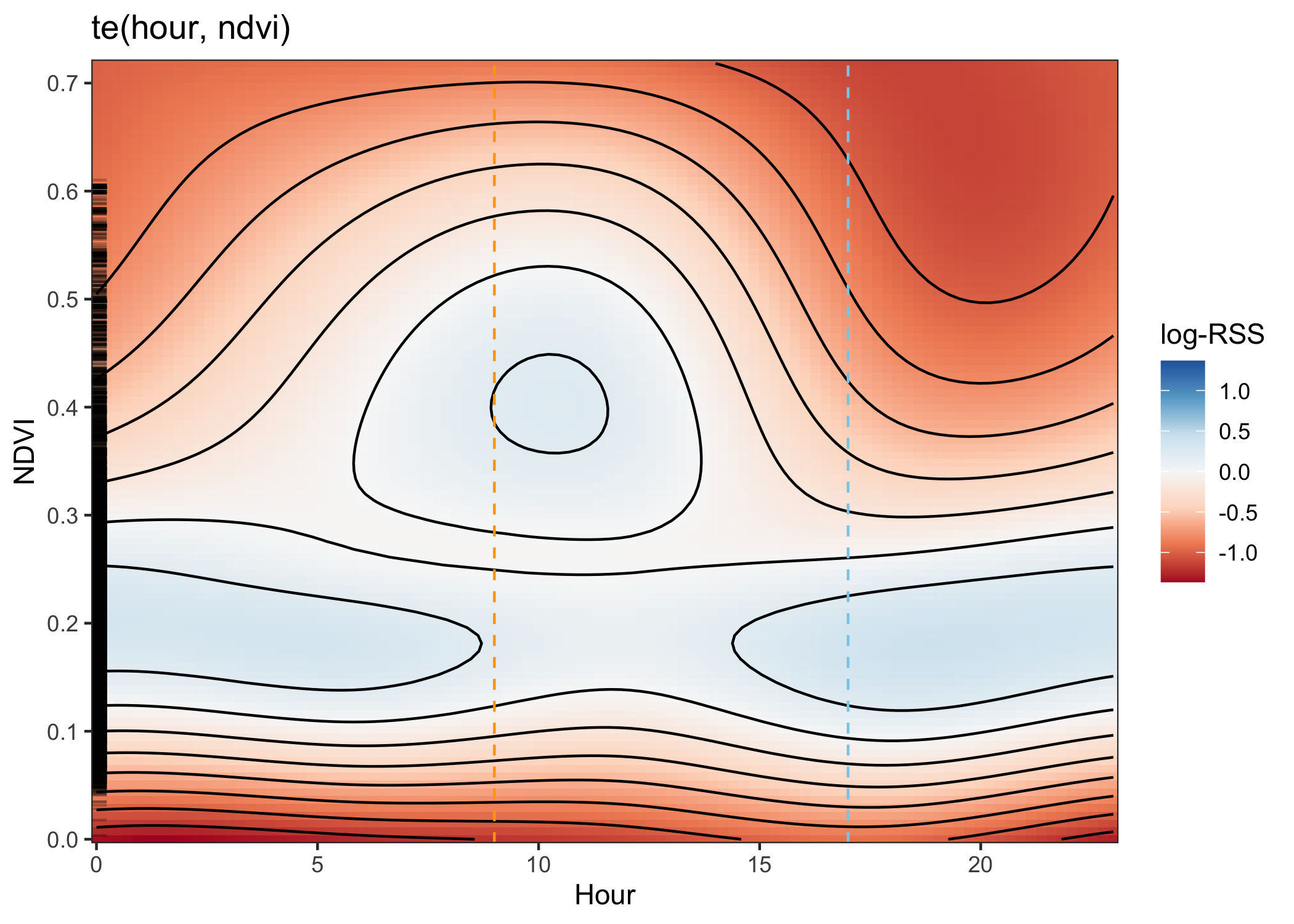

Code

ggsave(paste0(plot_save_path, "/ndvi_tensor_gam_response_id", which_buffalo, ".png"),
       width = 150, height = 80, units = "mm", dpi = 600)

Pull out a response curve from one of the hours

Code

# Get predictions on log-scale with standard errors
predictions <- predict(ssf_gam2d_temporal2, 
                      newdata = pred_data_hour9_17, 
                      type = "link",  # log-scale
                      se.fit = TRUE)

pred_data_hour9_17 <- pred_data_hour9_17 %>% 
  mutate(
    # Extract log RSS and standard errors
    log_rss = predictions$fit,
    se_log_rss = predictions$se.fit,
    # Calculate confidence intervals on log-scale
    log_rss_lower = log_rss - 1.96 * se_log_rss,
    log_rss_upper = log_rss + 1.96 * se_log_rss,
    # Transform to RSS scale
    rss = exp(log_rss),
    rss_lower = exp(log_rss_lower),
    rss_upper = exp(log_rss_upper)
  )

# plot the response curve
ggplot(data = pred_data_hour9_17) +
  geom_hline(yintercept = 1, linetype = "dashed", colour = "grey") +
  geom_ribbon(aes(x = ndvi, 
                  ymin = rss_lower, ymax = rss_upper,
                  fill = as.factor(hour)), 
              alpha = 0.5) +
  geom_line(aes(x = ndvi, y = rss, colour = as.factor(hour)), 
            linewidth = 1) +
  geom_rug(data = buffalo_ssf_data %>% filter(case_ == T), 
           aes(x = ndvi), alpha = 0.25, sides="b") +
  scale_colour_manual(values = c("orange", "skyblue")) +
  scale_fill_manual(values = c("orange", "skyblue")) +
  scale_x_continuous(breaks = seq(-0.2, 0.8, by = 0.1)) +
  scale_y_continuous(limits = c(0, 5.5)) +
  labs(x = "NDVI", y = "RSS") +
  theme_classic() +
  theme(legend.position = "none")

Code

ggsave(paste0(plot_save_path, "/ndvi_gam2d_response_sample_hour_id", which_buffalo, ".png"),
       width = 70, height = 80, units = "mm", dpi = 600)

References

Klappstein, Natasha J, Théo Michelot, John Fieberg, Eric J Pedersen, and Joanna Mills Flemming. 2024. “Step selection functions with non‐linear and random effects.” Methods in Ecology and Evolution, ahead of print, June 24. https://doi.org/10.1111/2041-210x.14367.

Load required packages

Import data and clean

Create a step object

Plot the data spatially

Pick out a single individual

Import spatial covariate

Select local extent

Sample random steps to fit models

Different SSF formulations

Set RSS min and max values

Linear covariate

Model formula

Fit model

Response curve

Plot habitat selection

Quadratic covariate

Model formula

Fit model

Generate the response curve

Response curve

Plot habitat selection

Smooth term

Model formula

Fit model

ALternatively, generate the response curve with the predict function

Plot habitat selection

Temporal dynamics

Static model for comparison

Pull out a response curve from one of the hours

Fit harmonic model with quadratic terms

Create table of NDVI and hour values

Easier to get the curves with GAM predict function

Fit model

Generate the response curve

Harmonic regression

Fit model

Pull out the coefficent across time

Calculate confidence intervals across time and plot

Pull out a response curve from one of the hours

Manually create the selection surface

Create table of NDVI and hour values

Fit harmonic model with quadratic terms

Manually create the selection surface

Create table of NDVI and hour values

Pull out a response curve from one of the hours

Temporal dynamics with smooth terms

Pull out a response curve from one of the hours

GAM selection surface

Fit 2D GAM smooth

Plot the smooth selection surface

Pull out a response curve from one of the hours

References

ALternatively, generate the response curve with the `predict` function