Assessing environmental extrapolation

Author

Scott Forrest

Published

August 25, 2026

Abstract

Here we show how to assess extrapolation (in environmental space), using the the continuous Shape metric (Velazco et al. 2024).

Load required packages

Code

# remotes::install_github("sjevelazco/flexsdm")

library(tidyverse)
packages <- c("amt", "sf", "terra", "tictoc", "beepr", "flexsdm", "tmap", "patchwork", "ggspatial")
walk(packages, require, character.only = T)

Import data and clean

Code

buffalo_data <- read_csv("data/buffalo.csv")

New names:
Rows: 133161 Columns: 11
── Column specification
──────────────────────────────────────────────────────── Delimiter: "," chr
(2): node, dates dbl (7): ...1, lat, lon, height, accuracy, heading, speed dttm
(2): timestamp, DateTime
ℹ Use `spec()` to retrieve the full column specification for this data. ℹ
Specify the column types or set `show_col_types = FALSE` to quiet this message.
• `` -> `...1`

Code

# remove individuals that have poor data quality or less than about 3 months of data. 
# The "2014.GPS_COMPACT copy.csv" string is a duplicate of ID 2024, so we exclude it
buffalo_data <- buffalo_data %>% filter(!node %in% c("2014.GPS_COMPACT copy.csv", 
                                           2029, 2043, 2265, 2284, 2346))

buffalo_data <- buffalo_data %>%  
  group_by(node) %>% 
  arrange(DateTime, .by_group = T) %>% 
  distinct(DateTime, .keep_all = T) %>% 
  arrange(node) %>% 
  mutate(ID = node)

buffalo_clean <- buffalo_data[, c(12, 2, 4, 3)]
colnames(buffalo_clean) <- c("id", "time", "lon", "lat")
attr(buffalo_clean$time, "tzone") <- "Australia/Queensland"
buffalo_clean$sex <- "f"
buffalo_clean$life_stage <- "adult"
head(buffalo_clean)

Code

tz(buffalo_clean$time)

[1] "Australia/Queensland"

Code

buffalo_ids <- unique(buffalo_clean$id)

write_csv(buffalo_clean, "data/buffalo_clean.csv")

Create a step object

Use the amt package to create a trajectory object from the cleaned data.

Create a trajectory object

buffalo_all <- buffalo_clean %>% mk_track(id = id,
                                           lon,
                                           lat, 
                                           time, 
                                           all_cols = T,
                                           crs = 4326) %>% 
  transform_coords(crs_to = 3112, crs_from = 4326) # Transformation to GDA94 / 
# Geoscience Australia Lambert (https://epsg.io/3112)

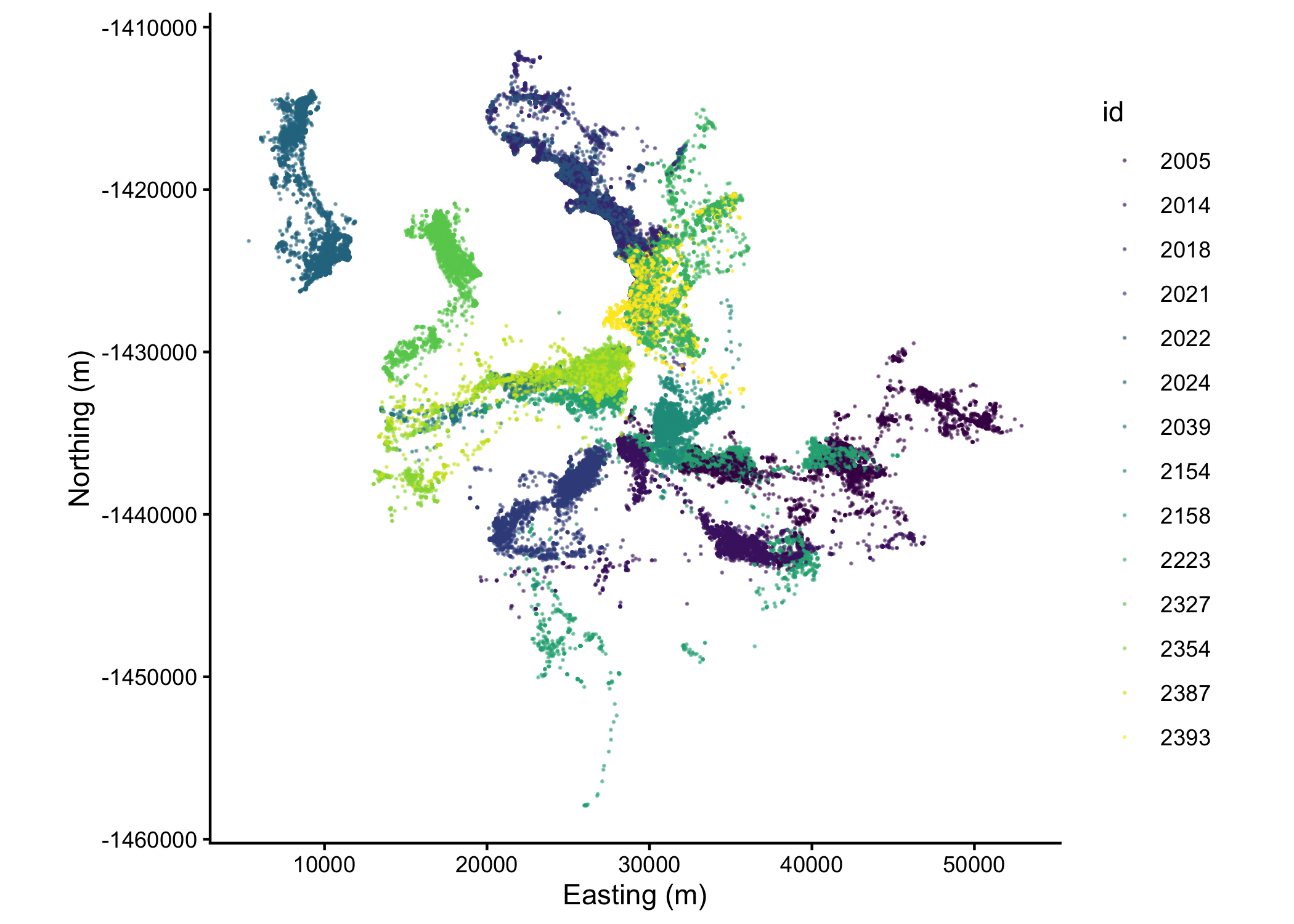
Plot the data spatially

Code

buffalo_all %>%
  ggplot(aes(x = x_, y = y_, colour = id)) +
  geom_point(alpha = 0.5, size = 0.1) + 
  coord_fixed() +
  scale_x_continuous("Easting (m)") +
  scale_y_continuous("Northing (m)") +
  scale_colour_viridis_d() +
  theme_classic() +
  theme(legend.position = "right")

Code

# ggsave("outputs/data_prep/buffalo_djelk_map.png",
#        width = 150, height = 150, units = "mm",  dpi = 600)

Creating a step object

Create steps

# nest the data by individual
buffalo_all_nested <- buffalo_all %>% arrange(id) %>% nest(data = -"id")

buffalo_all_nested_steps <- buffalo_all_nested %>%
  mutate(steps = map(data, function(x)
    x %>% track_resample(rate = hours(1), tolerance = minutes(10)) %>%
      steps()))

Warning: There were 14 warnings in `mutate()`.
The first warning was:
ℹ In argument: `steps = map(...)`.
Caused by warning in `steps.track_xyt()`:
! burst's are ignored, use steps_by_burst instead.
ℹ Run `dplyr::last_dplyr_warnings()` to see the 13 remaining warnings.

Create steps

# unnest the data after creating 'steps' objects
buffalo_all_steps <- buffalo_all_nested_steps %>% 
  amt::select(id, steps) %>% 
  amt::unnest(cols = steps)

buffalo_all_steps <- buffalo_all_steps %>% 
  mutate(t2_rounded = round_date(t2_, "hour"), # round the time to the nearest hour
         hour_t2 = ifelse(hour(t2_rounded) == 0, 24, hour(t2_rounded))) # change the 0 hour to 24

head(buffalo_all_steps, 10)

Fitting step length and turning angle distributions

Fitting exponential and von Mises distributions to the steps of ALL individuals (only one Gamma and one von Mises distribution for the whole population). This should be done when fitting a hierarchical model to update the ‘population’ parameters, but also makes it straightforward to update after model fitting to each individual separately.

Fit step length and turning angle distributions

# fitting step length and turning angle distributions to all locations
gamma_dist <- fit_distr(buffalo_all_steps$sl_, "gamma")
vonmises_dist <- fit_distr(buffalo_all_steps$ta_, "vonmises")

# checking parameters - which can then be saved to update movement parameters 
# after fitting the step selection model
gamma_dist$params$shape

[1] 0.4266711

Fit step length and turning angle distributions

gamma_dist$params$scale

[1] 664.0039

Fit step length and turning angle distributions

vonmises_dist$params$kappa

[1] 0.1990268

Fit step length and turning angle distributions

vonmises_dist$params$mu

Circular Data: 
Type = angles 
Units = radians 
Template = none 
Modulo = asis 
Zero = 0 
Rotation = counter 
[1] 0

For some reason, the random_steps function does not work when using the bursted_steps_xyt class. I’m not sure why (the error is Error in bursts[[i]] : subscript out of bounds), but it works when that class label is removed, and appears to sample random steps correctly. For taxa that have irregular fixes and many bursts, this may be worth exploring in more detail.

Create random steps

tic()

buffalo_parametric_popn_GvM <- buffalo_all_steps %>% 
  random_steps(n_control = 10,
               sl_distr = gamma_dist,
               ta_distr = vonmises_dist) %>% 
  mutate(y = as.numeric(case_))

toc()

13.51 sec elapsed

Plotting the random step distributions

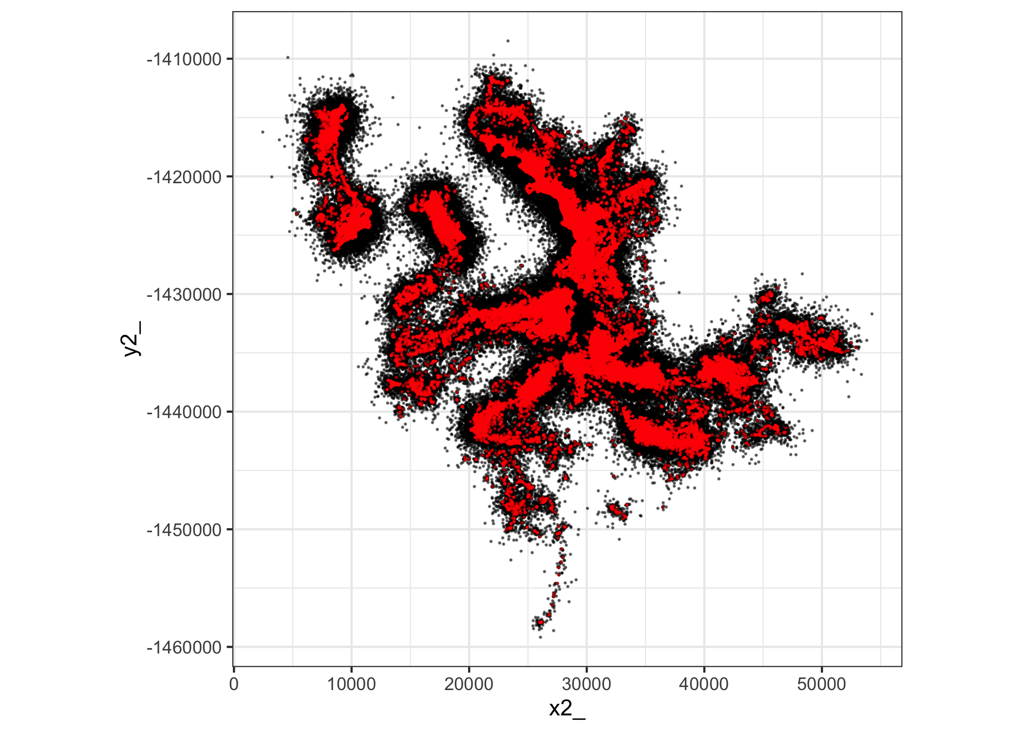
Spatially plot the used and random steps, with the used steps in red.

Plot the random steps

buffalo_parametric_popn_GvM %>% ggplot() +
  geom_point(data = . %>% filter(y == 0), aes(x = x2_, y = y2_), 
             colour = "black", size = 0.1, alpha = 0.5) +
  geom_point(data = . %>% filter(y == 1), aes(x = x2_, y = y2_), 
             colour = "red", size = 0.1, alpha = 0.5) +
  coord_equal() +
  theme_bw()

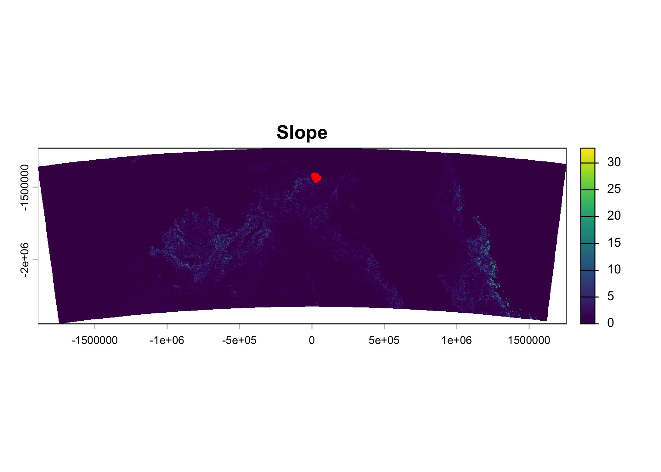
Import spatial covariates

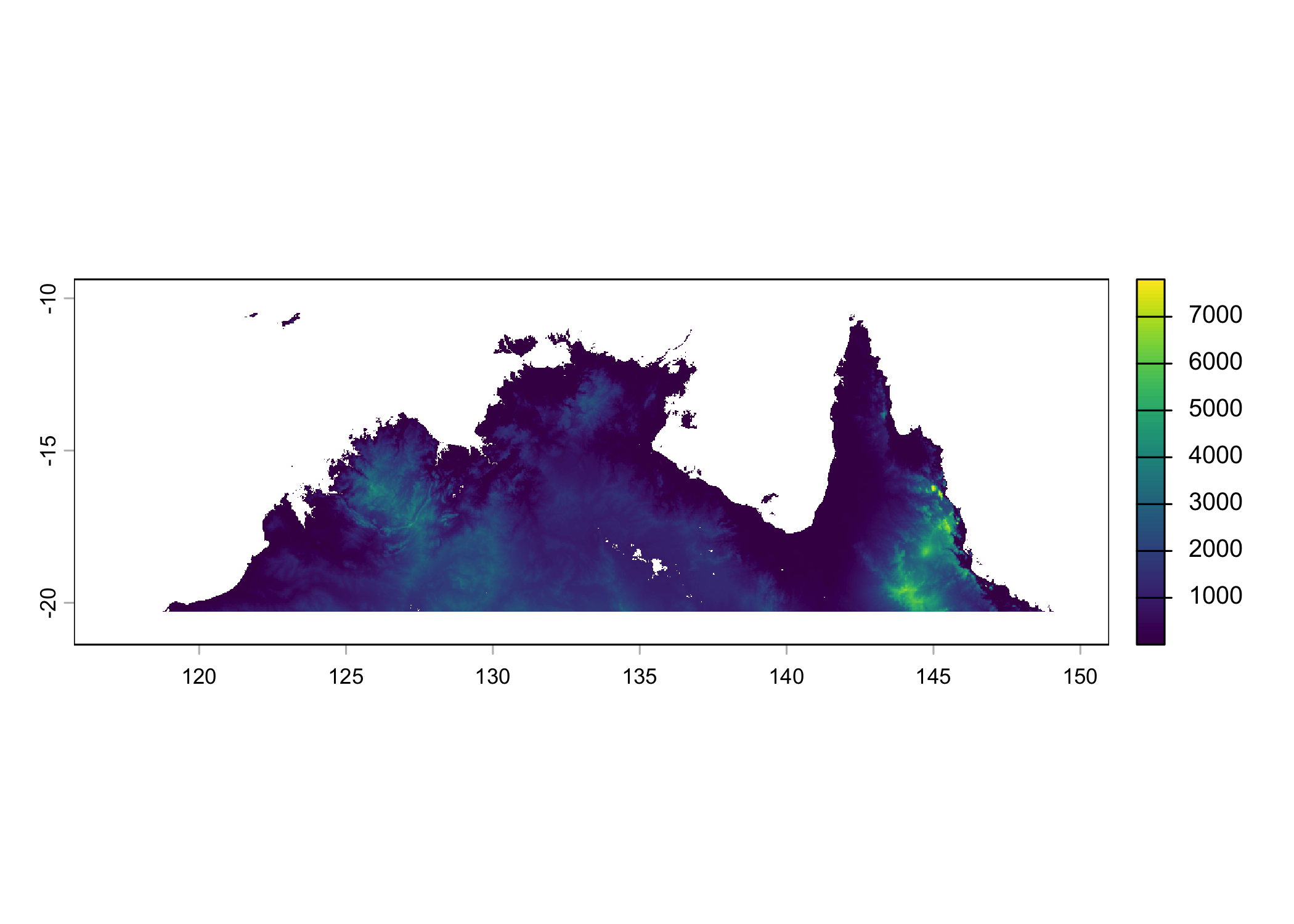
Although NDVI changes over time, and we have access to monthly layers, we will just select a single month here.

Code

# NDVI
# ndvi <- terra::rast("mapping/large_files/NDVI_2023_250m.tif")
# ndvi <- terra::project(ndvi, "EPSG:3112")
# writeRaster(ndvi, "mapping/large_files/NDVI_2023_250m_projected3112.tif", overwrite = TRUE)

ndvi <- terra::rast("mapping/large_files/NDVI_2023_250m_projected3112.tif")
plot(ndvi, main = "NDVI July 2023")
points(buffalo_all$x_, buffalo_all$y_, col = "red", pch = 16, cex = 0.5)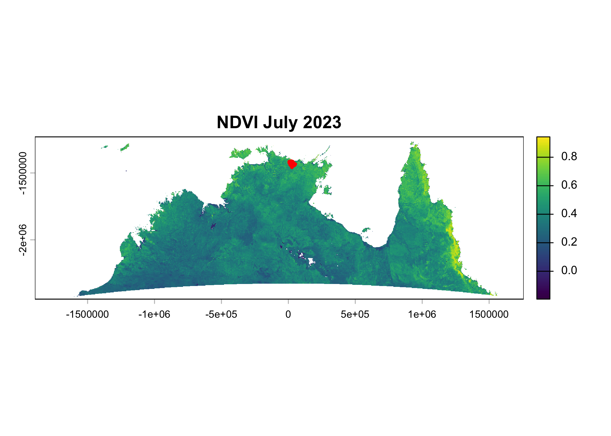

Code

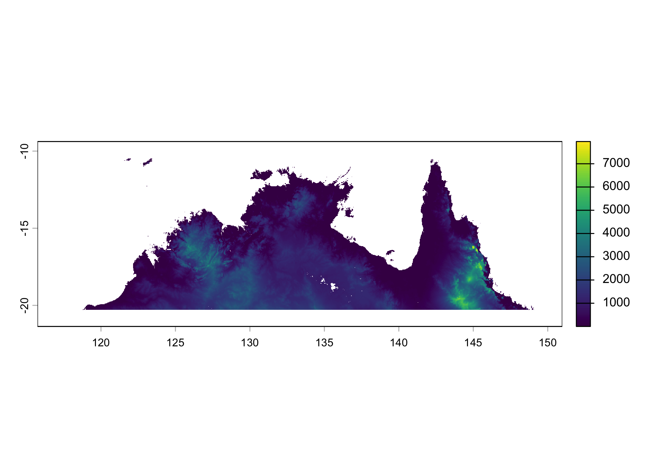
# elevation
# elev <- terra::rast("mapping/large_files/DEM_SRTM_250m.tif")
# elev <- terra::project(elev, "EPSG:3112")
# writeRaster(elev, "mapping/large_files/DEM_SRTM_250m_projected3112.tif", overwrite = TRUE)

elev <- terra::rast("mapping/large_files/DEM_SRTM_250m_projected3112.tif")
plot(elev, main = "Elevation")
points(buffalo_all$x_, buffalo_all$y_, col = "red", pch = 16, cex = 0.5)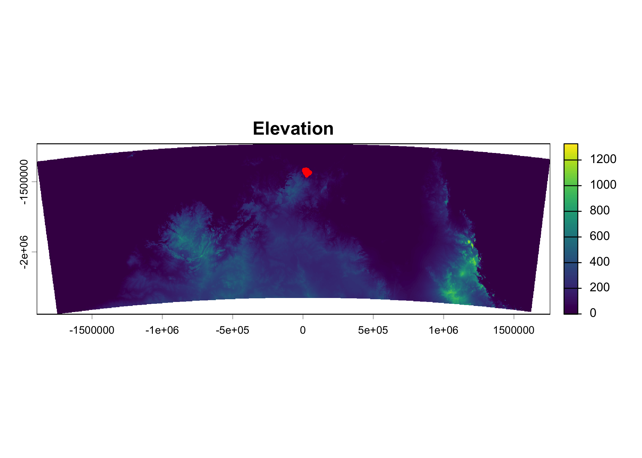

Code

# create slope layer
slope <- terra::terrain(elev, v = "slope", neighbors = 8)
plot(slope, main = "Slope")
points(buffalo_all$x_, buffalo_all$y_, col = "red", pch = 16, cex = 0.5)

Sample values of the environmental covariates at the end of the steps.

Extract covariates at the end of the steps

buffalo_parametric_popn_covs <- buffalo_parametric_popn_GvM %>% 
  
  extract_covariates(ndvi,
                     where = "end") %>%
  extract_covariates(elev,
                     where = "end") %>%
  extract_covariates(slope,
                     where = "end") %>% 
  
  mutate(y = as.numeric(case_),
         cos_ta_ = cos(ta_),
         log_sl_ = log(sl_))

Assess extrapolation

Code

# uncomment to run the code - takes a while
# tic()
# 
# extrapolation_raster <- extra_eval(
#   training_data = buffalo_parametric_popn_covs,
#   pr_ab = "y",
#   projection_data = c(ndvi, elev, slope), 
#   metric = "mahalanobis",
#   univar_comb = FALSE,
#   aggreg_factor = 10
# )
# 
# beep(sound = 2)
# 
# toc()

Write the raster

Code

# terra::writeRaster(extrapolation_raster, "outputs/extrapolation_raster.tif", overwrite = TRUE)
extrapolation_raster <- terra::rast("outputs/extrapolation_raster.tif")

Mask out NAs and plot

Code

extrapolation_raster <- terra::mask(extrapolation_raster, ndvi)
extrapolation_raster_wgs84 <- terra::project(extrapolation_raster, "EPSG:4326")
plot(extrapolation_raster_wgs84)

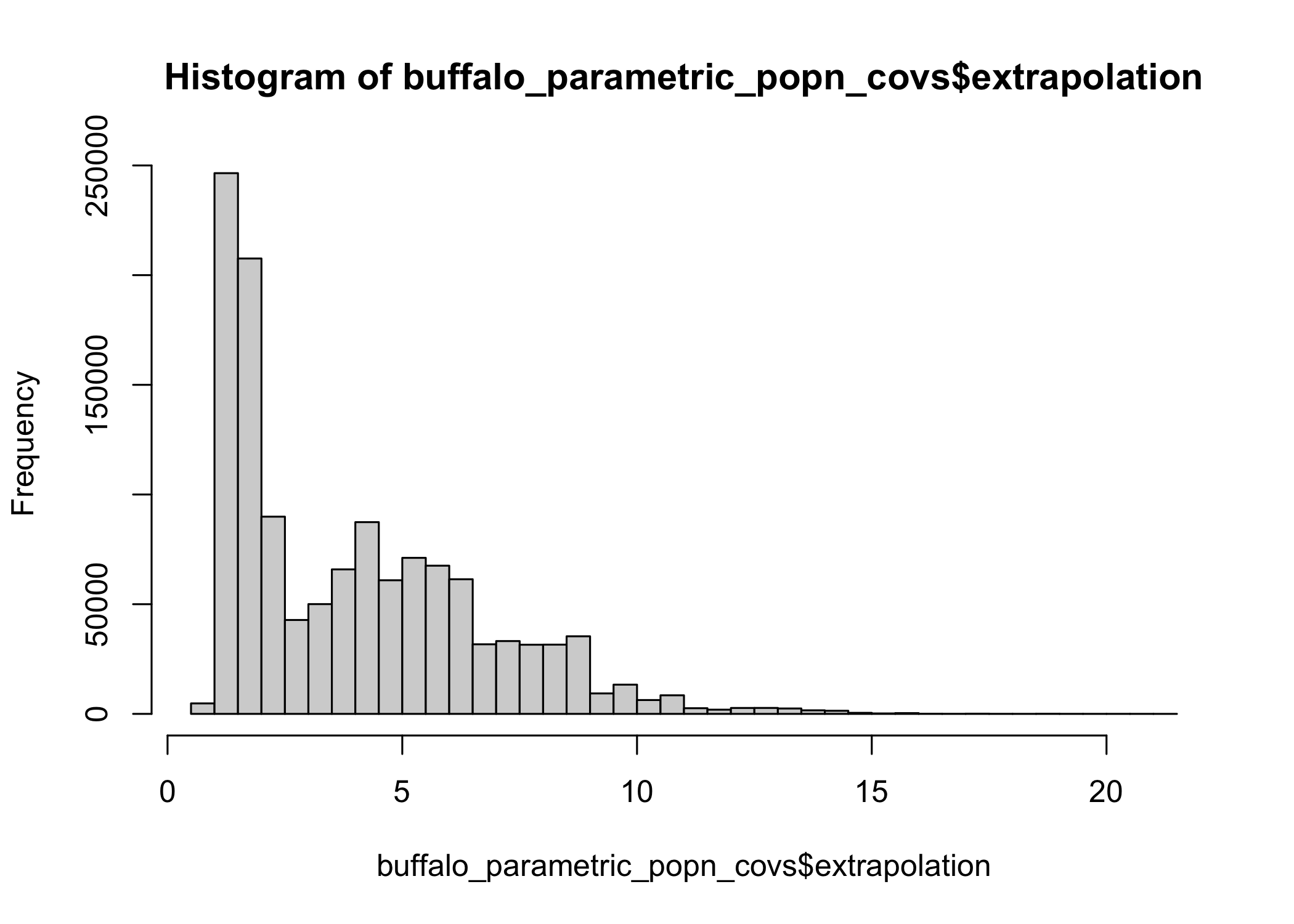
Add Shape values back to the training dataframe

Code

buffalo_parametric_popn_covs <- buffalo_parametric_popn_covs %>% 
  extract_covariates(extrapolation_raster,
                     where = "end")

hist(buffalo_parametric_popn_covs$extrapolation, breaks = 30)

Code

# what is the 99th percentile of the Shape values in the training data?
threshold_q99 <- quantile(buffalo_parametric_popn_covs$extrapolation, 0.99, na.rm = TRUE)
paste0("The 99th percentile of the Shape values in the training data is ", threshold_q99)

[1] "The 99th percentile of the Shape values in the training data is 11.8537864685059"

Code

# what is the maximum Shape value in the training data?
threshold_max <- max(buffalo_parametric_popn_covs$extrapolation, na.rm = TRUE)
paste0("The maximum Shape value in the training data is ", threshold_max)

[1] "The maximum Shape value in the training data is 21.1267185211182"

Plot histogram of Shape values in the training data with the 99th percentile and maximum values indicated

Code

ggplot() +
  geom_histogram(data = buffalo_parametric_popn_covs, aes(x = extrapolation), 
                 fill = "orange", colour = "black", bins = 30) +
  geom_vline(xintercept = threshold_q99, color = "red", linetype = "dashed") +
  geom_vline(xintercept = threshold_max, color = "red", linetype = "dashed") +
  labs(x = "Extrapolation (Shape)", y = "Frequency") +
  theme_bw()

Warning: Removed 64 rows containing non-finite outside the scale range
(`stat_bin()`).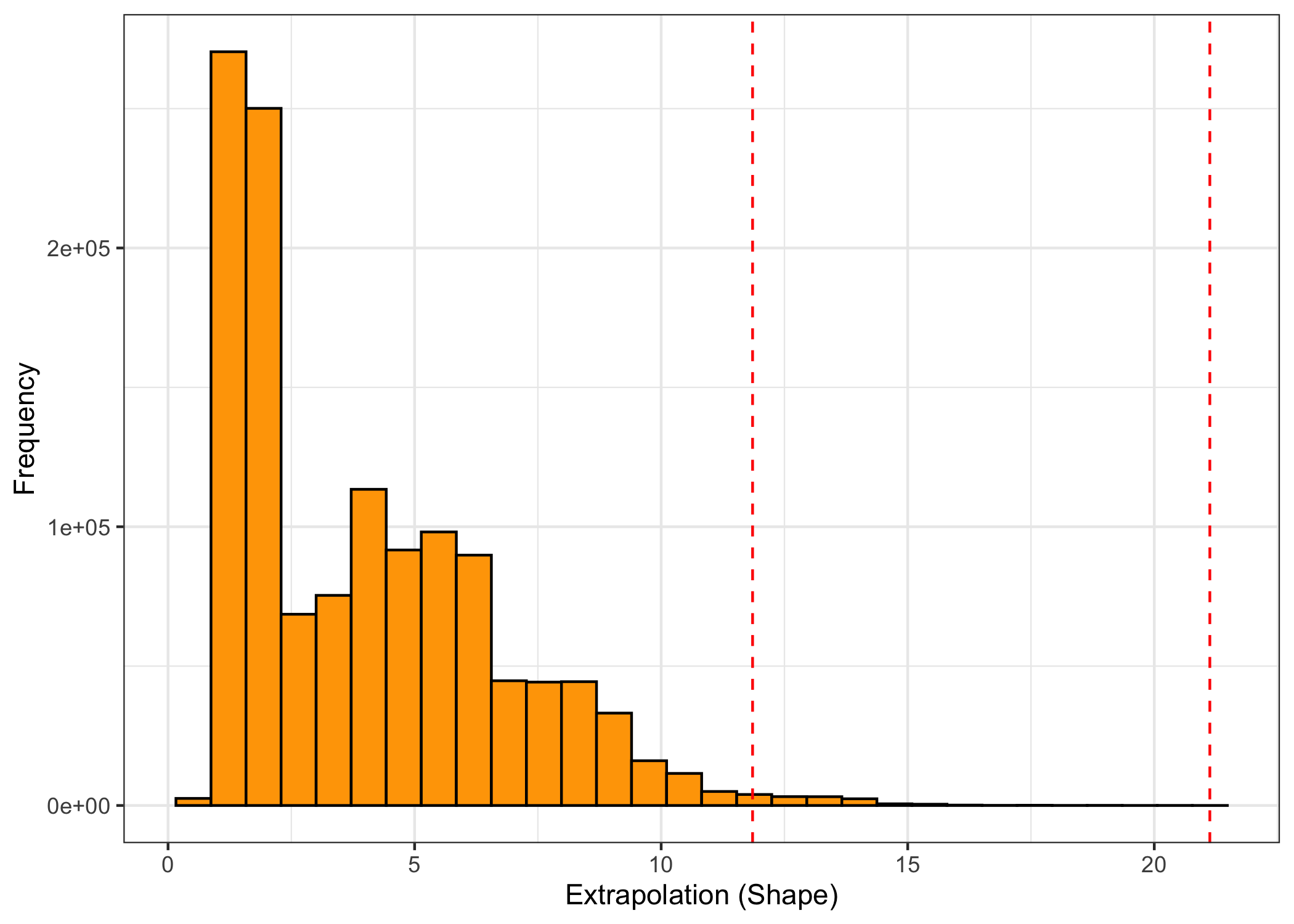

Plot the extrapolation

Create dataframe

Code

# prevent scientific notation in the legend
options(scipen=999)

extrapolation_raster_wgs84_agg <- terra::aggregate(extrapolation_raster_wgs84, fact = 4, fun = mean)


|---------|---------|---------|---------|
=========================================

Code

plot(extrapolation_raster_wgs84_agg)

Code

extrapolation_raster_wgs84_agg_df <- as.data.frame(extrapolation_raster_wgs84_agg, xy = TRUE)

Thin the training data

Code

buffalo_parametric_popn_covs_thin <- buffalo_parametric_popn_covs %>% dplyr::slice_sample(prop = 1)

# project to WGS84 for plotting with ggplot
xy_wgs84 <- buffalo_parametric_popn_covs_thin %>%
  st_as_sf(coords = c("x1_", "y1_"), crs = 3112) %>%
  st_transform(crs = 4326) %>%
  st_coordinates() %>%
  as.data.frame() %>%
  rename(x1_wgs84 = X, y1_wgs84 = Y)

buffalo_parametric_popn_covs_thin <- buffalo_parametric_popn_covs_thin %>%
  bind_cols(xy_wgs84)

Plot with ggplot

Code

raster_alpha <- 0.5
training_points_alpha <- 0.1

extrapolation_aus_plot <- ggplot(data = extrapolation_raster_wgs84_agg_df, aes(x = x, y = y, fill = extrapolation)) +
  
  geom_raster() +
    scale_fill_viridis_c(
    na.value = "transparent",
    transform = "log1p",
    breaks = c(1, 10, 100, 1000, 5000)
  ) +
  
  geom_contour(aes(z = extrapolation),
               breaks = c(threshold_max), color = "orange", linewidth = 0.2) +
  
  geom_point(data = buffalo_parametric_popn_covs_thin,
             aes(x = x1_wgs84, y = y1_wgs84),
             colour = "red", alpha = training_points_alpha, size = 0.01) +
  
  annotation_scale(location = "bl", width_hint = 0.2) +
  coord_sf(crs = 4326, default_crs = 4326, expand = FALSE) +
  labs(x = NULL, y = NULL, fill = "Extrapolation\n(Shape)") +
  theme_classic() +
  theme(
    legend.position = "inside",
    legend.position.inside = c(0.95, 0.7)
    )

extrapolation_aus_plot

Warning: The following aesthetics were dropped during statistical transformation: fill.
ℹ This can happen when ggplot fails to infer the correct grouping structure in
  the data.
ℹ Did you forget to specify a `group` aesthetic or to convert a numerical
  variable into a factor?

Warning: Raster pixels are placed at uneven horizontal intervals and will be shifted
ℹ Consider using `geom_tile()` instead.

`geom_raster()` only works with linear coordinate systems, not `coord_sf()`.
ℹ Falling back to drawing as `geom_rect()`.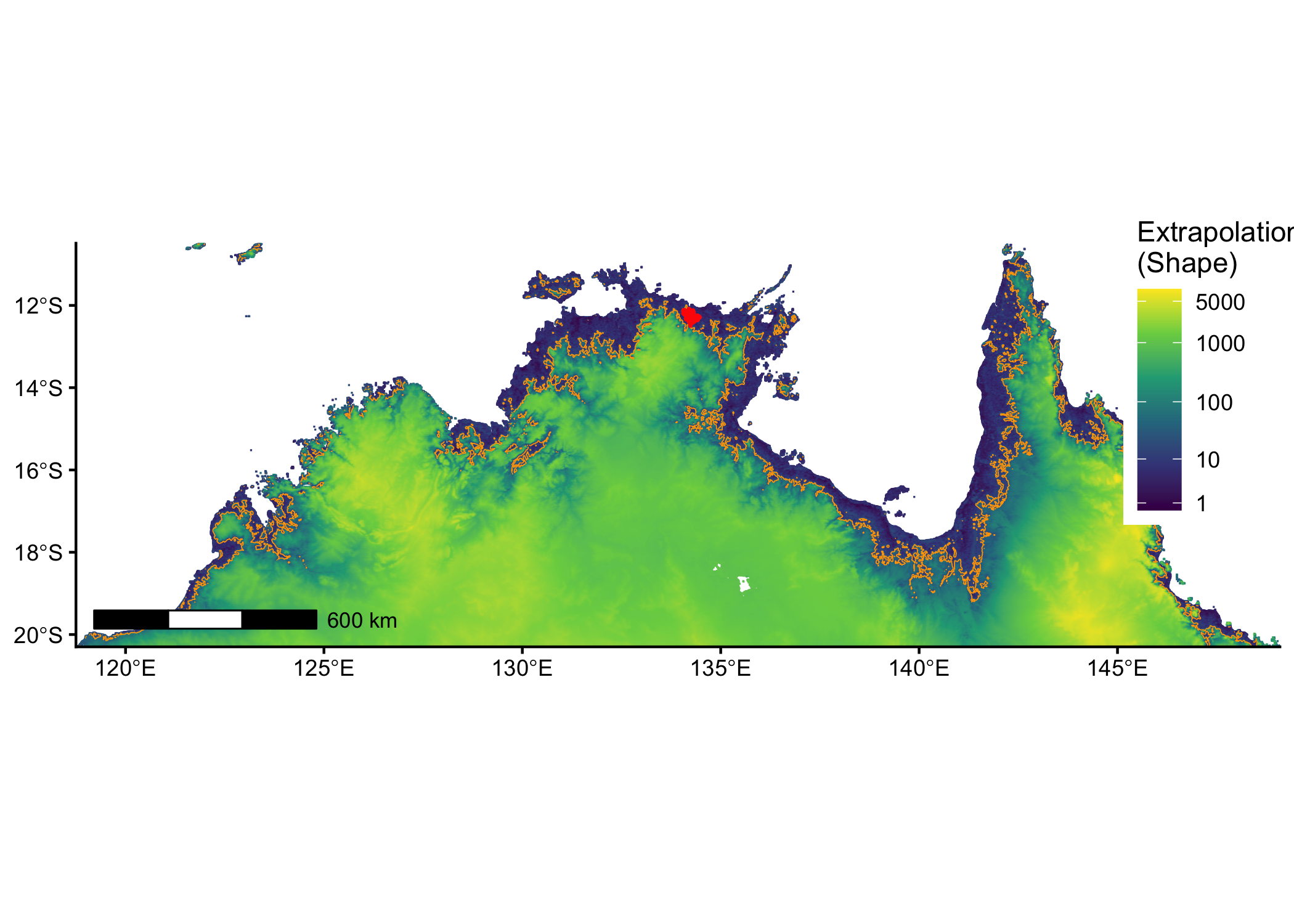

Code

ggsave("outputs/extrapolation_raster_ggplot.png",
       width = 180, height = 60, units = "mm", scale = 1.5, dpi = 1000)

Warning: The following aesthetics were dropped during statistical transformation: fill.
ℹ This can happen when ggplot fails to infer the correct grouping structure in
  the data.
ℹ Did you forget to specify a `group` aesthetic or to convert a numerical
  variable into a factor?
Raster pixels are placed at uneven horizontal intervals and will be shifted
ℹ Consider using `geom_tile()` instead.

`geom_raster()` only works with linear coordinate systems, not `coord_sf()`.
ℹ Falling back to drawing as `geom_rect()`.

Check distributions of covariates against Shape values

Code

cov_extrap_stack <- c(ndvi, elev, slope, extrapolation_raster)
cov_extrap_stack_df <- as.data.frame(cov_extrap_stack, xy = TRUE) %>% drop_na()

# thin to reduce computation and make plot look less messy
cov_extrap_stack_df_thin <- cov_extrap_stack_df %>% dplyr::slice_sample(prop = 0.001)

Plot NDVI and elevation with Shape values

Code

ndvi_elev_plot <- ggplot() +
  
  geom_point(data = cov_extrap_stack_df_thin, 
             aes(x = NDVI, y = elevation, colour = extrapolation), alpha = raster_alpha) +
  
  geom_point(data = buffalo_parametric_popn_covs_thin,
             aes(x = NDVI, y = elevation),
             colour = "red", alpha = training_points_alpha) +
  
  scale_colour_viridis_c(
    transform = "log1p",
    breaks = c(1, 10, 100, 1000, 5000)
    ) +
  
  labs(x = "NDVI", y = "Elevation", colour = "Extrapolation\n(Shape)")  +
  theme_classic() +
  theme(legend.position = "none")

ndvi_elev_plot

Warning: Removed 64 rows containing missing values or values outside the scale range
(`geom_point()`).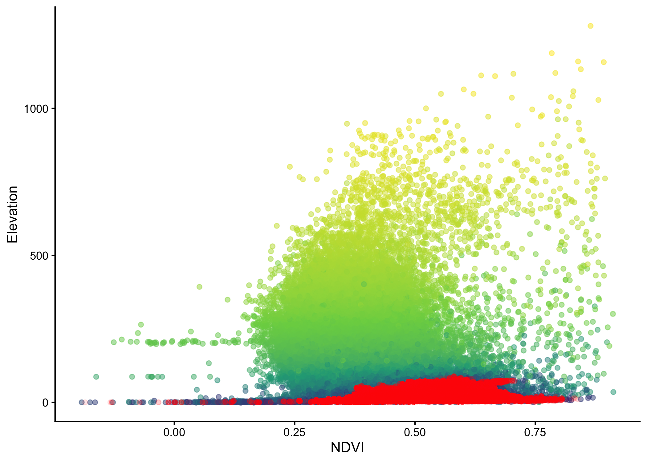

Plot NDVI and slope with Shape values

Code

ndvi_slope_plot <- ggplot() +
  
  geom_point(data = cov_extrap_stack_df_thin, 
             aes(x = NDVI, y = slope, colour = extrapolation), alpha = raster_alpha) +
  
  geom_point(data = buffalo_parametric_popn_covs_thin,
             aes(x = NDVI, y = slope),
             colour = "red", alpha = training_points_alpha) +
  
  scale_colour_viridis_c(
    transform = "log1p",
    breaks = c(1, 10, 100, 1000, 5000)
    ) +
  
  labs(x = "NDVI", y = "Slope", colour = "Extrapolation\n(Shape)") +
  theme_classic() +
  theme(legend.position = "none")

ndvi_slope_plot

Warning: Removed 64 rows containing missing values or values outside the scale range
(`geom_point()`).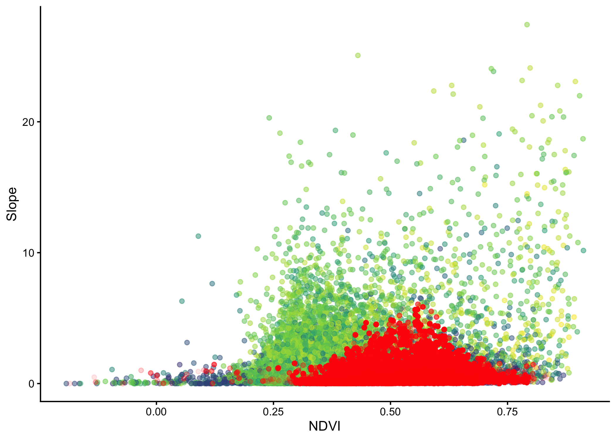

Plot elevation and slope with Shape values

Code

elev_slope_plot <- ggplot() +
  
  geom_point(data = cov_extrap_stack_df_thin, 
             aes(x = elevation, y = slope, colour = extrapolation), alpha = raster_alpha) +
  
  geom_point(data = buffalo_parametric_popn_covs_thin,
             aes(x = elevation, y = slope),
             colour = "red", alpha = training_points_alpha) +
  
  scale_colour_viridis_c(
    transform = "log1p",
    breaks = c(1, 10, 100, 1000, 5000)
    ) +
  
  labs(x = "Elevation", y = "Slope", colour = "Extrapolation\n(Shape)") +
  theme_classic() +
  theme(legend.position = "none")

elev_slope_plot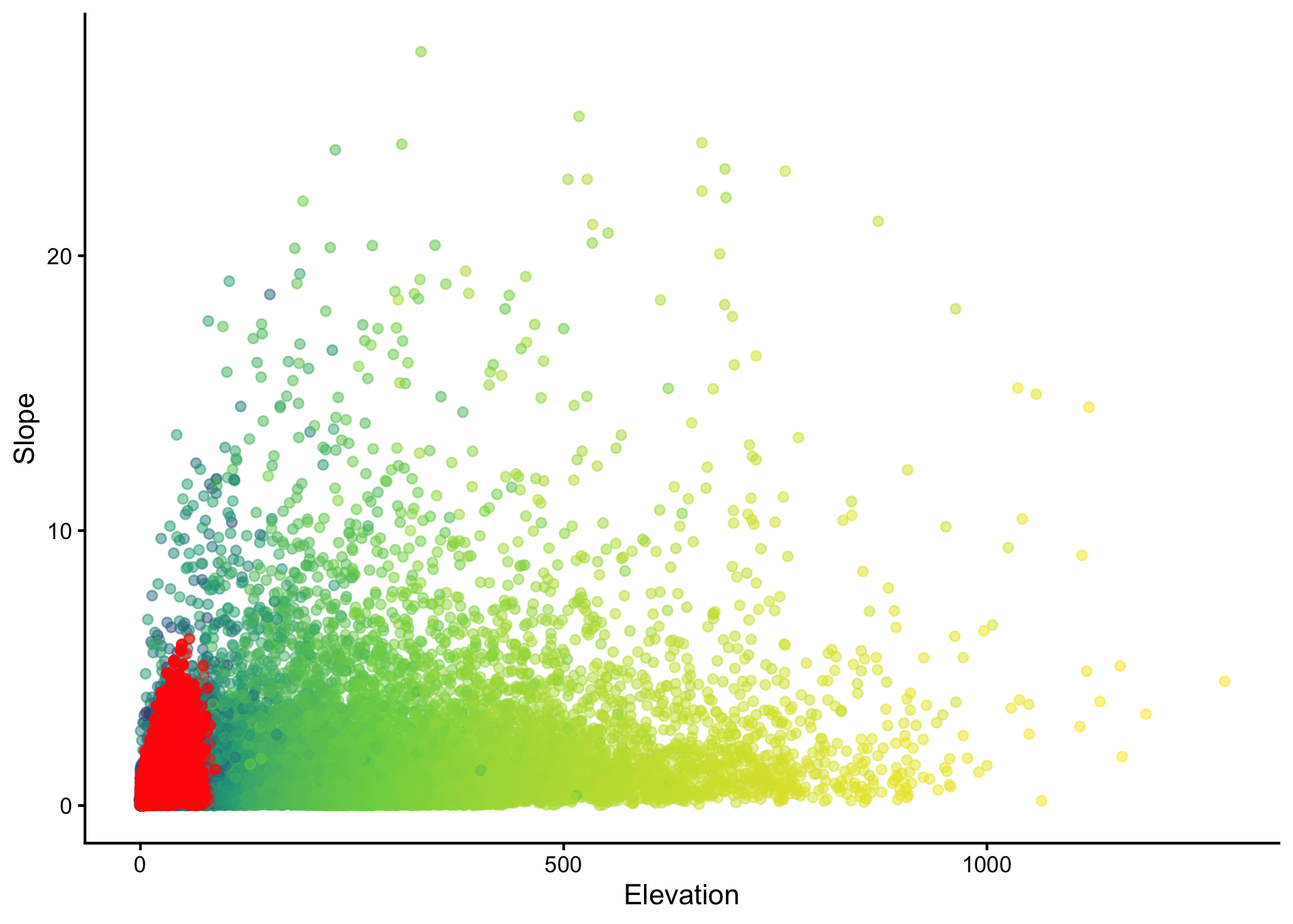

Combine the plots

Code

extrapolation_aus_plot / 
  (ndvi_elev_plot | ndvi_slope_plot | elev_slope_plot) +
  plot_layout(heights = c(2, 1)) #+

Warning: The following aesthetics were dropped during statistical transformation: fill.
ℹ This can happen when ggplot fails to infer the correct grouping structure in
  the data.
ℹ Did you forget to specify a `group` aesthetic or to convert a numerical
  variable into a factor?

Warning: Raster pixels are placed at uneven horizontal intervals and will be shifted
ℹ Consider using `geom_tile()` instead.

`geom_raster()` only works with linear coordinate systems, not `coord_sf()`.
ℹ Falling back to drawing as `geom_rect()`.

Warning: Removed 64 rows containing missing values or values outside the scale range
(`geom_point()`).

Warning: Removed 64 rows containing missing values or values outside the scale range
(`geom_point()`).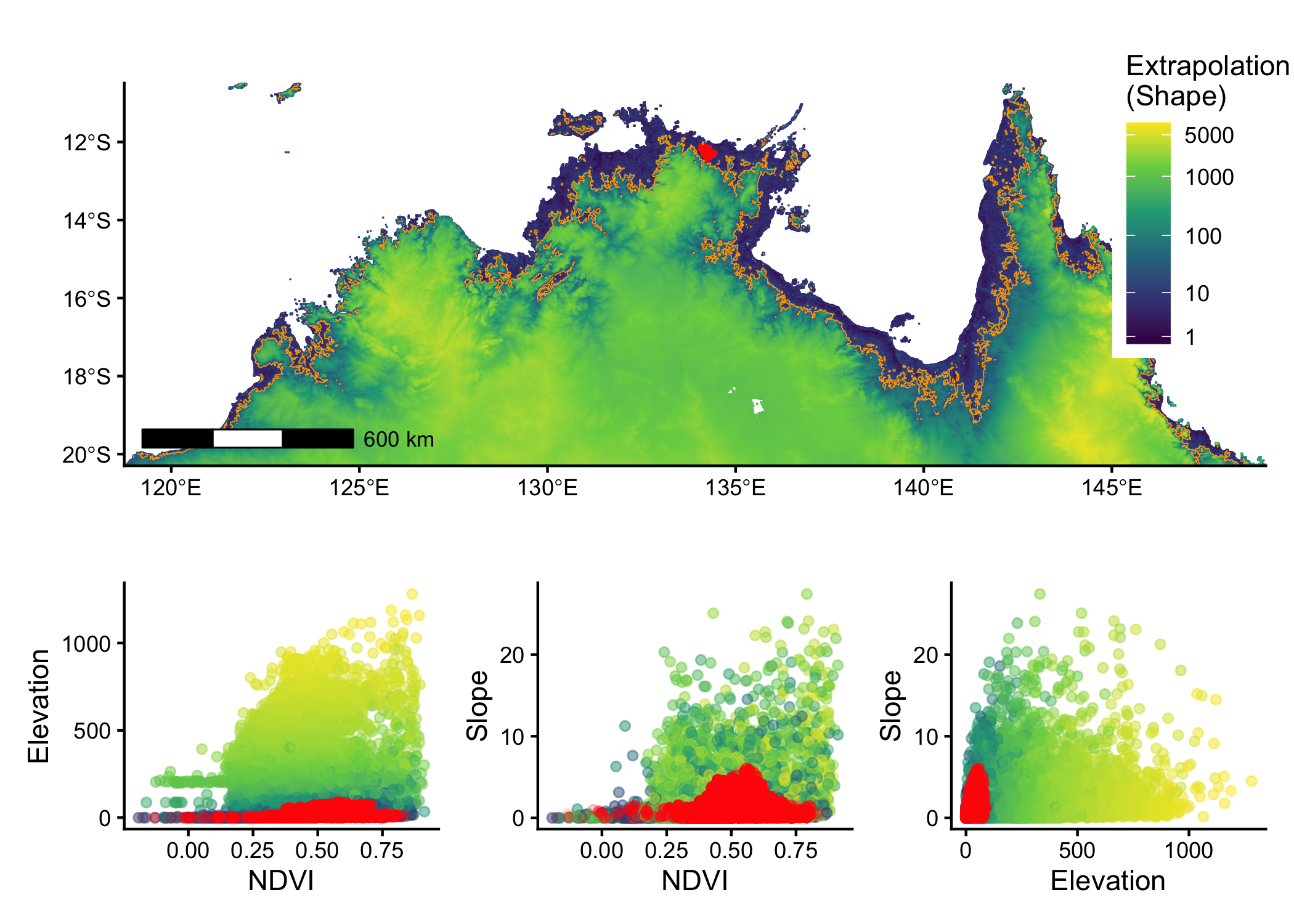

Code

  # plot_annotation(tag_levels = "A")

ggsave("outputs/extrapolation_aus_covs.png",
       width = 180, height = 110, units = "mm", scale = 1.5, dpi = 600)

Warning: The following aesthetics were dropped during statistical transformation: fill.
ℹ This can happen when ggplot fails to infer the correct grouping structure in
  the data.
ℹ Did you forget to specify a `group` aesthetic or to convert a numerical
  variable into a factor?

Warning: Raster pixels are placed at uneven horizontal intervals and will be shifted
ℹ Consider using `geom_tile()` instead.

`geom_raster()` only works with linear coordinate systems, not `coord_sf()`.
ℹ Falling back to drawing as `geom_rect()`.

Warning: Removed 64 rows containing missing values or values outside the scale range
(`geom_point()`).

Warning: Removed 64 rows containing missing values or values outside the scale range
(`geom_point()`).

Create zoomed plot for earlier figure

Crop spatial covariates

Code

# set the extent
zoom_extent_min_x <- min(buffalo_parametric_popn_covs_thin$x1_) - 20000
zoom_extent_max_x <- max(buffalo_parametric_popn_covs_thin$x1_) + 120000
zoom_extent_min_y <- min(buffalo_parametric_popn_covs_thin$y1_) - 50000
zoom_extent_max_y <- max(buffalo_parametric_popn_covs_thin$y1_) + 20000

# create extent
crop_extent <- terra::ext(
  zoom_extent_min_x,
  zoom_extent_max_x,
  zoom_extent_min_y,
  zoom_extent_max_y
)

ndvi_crop <- terra::crop(ndvi, crop_extent)
elev_crop <- terra::crop(elev, crop_extent)
slope_crop <- terra::crop(slope, crop_extent)

Assess extrapolation

Code

# commented out here as it takes about 45 minutes to run
# tic()
# 
# extrapolation_raster_crop <- extra_eval(
#   training_data = buffalo_parametric_popn_covs,
#   pr_ab = "y",
#   projection_data = c(ndvi_crop, elev_crop, slope_crop),
#   metric = "mahalanobis",
#   univar_comb = FALSE,
#   aggreg_factor = 1
# )
# 
# beep(sound = 2)
# 
# toc()

# terra::writeRaster(extrapolation_raster_crop, "outputs/extrapolation_raster_crop.tif", overwrite = TRUE)
extrapolation_raster_crop <- terra::rast("outputs/extrapolation_raster_crop.tif")

Code

# mask and create dataframe for plotting
extrapolation_raster_crop <- terra::mask(extrapolation_raster_crop, ndvi_crop)
extrapolation_raster_cropped_df <- as.data.frame(extrapolation_raster_crop, xy = TRUE)

# plot with ggplot
ggplot(data = extrapolation_raster_cropped_df, aes(x = x, y = y, fill = extrapolation)) +
  
  geom_raster() +
  
  scale_fill_viridis_c(
    na.value = "transparent",
    transform = "log1p",
    breaks = c(1, 10, 100, 500)
  ) +
  
  geom_contour(aes(z = extrapolation),
               breaks = c(threshold_max), color = "orange", linewidth = 0.3) +
  
  # geom_point(data = buffalo_parametric_popn_covs %>% filter(y == 0),
  #            aes(x = x2_, y = y2_),
  #            colour = "black", alpha = 0.25, size = 0.01) +
  
  geom_point(data = buffalo_parametric_popn_covs %>% filter(y == 1),
             aes(x = x1_, y = y1_),
             colour = "red", alpha = 0.25, size = 0.01) +
  
  annotation_scale(location = "bl", width_hint = 0.2) +
  coord_sf(crs = 3112, default_crs = 3112, expand = FALSE) +
  labs(x = NULL, y = NULL, fill = "Extrapolation\n(Shape)") +
  theme_classic() +
  theme(
    legend.position = "right"
    )

Warning: The following aesthetics were dropped during statistical transformation: fill.
ℹ This can happen when ggplot fails to infer the correct grouping structure in
  the data.
ℹ Did you forget to specify a `group` aesthetic or to convert a numerical
  variable into a factor?

`geom_raster()` only works with linear coordinate systems, not `coord_sf()`.
ℹ Falling back to drawing as `geom_rect()`.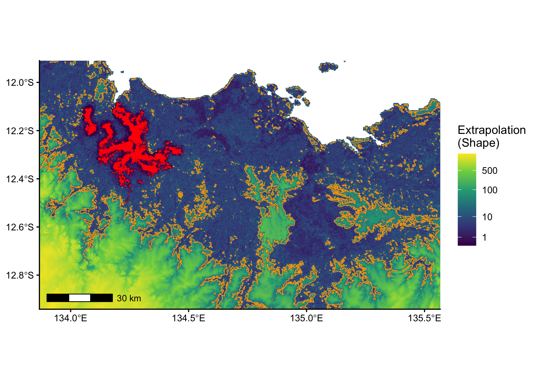

Code

ggsave("outputs/extrapolation_raster_cropped_ggplot.png",
       width = 180, height = 90, units = "mm", scale = 1.5, dpi = 600)

Warning: The following aesthetics were dropped during statistical transformation: fill.
ℹ This can happen when ggplot fails to infer the correct grouping structure in
  the data.
ℹ Did you forget to specify a `group` aesthetic or to convert a numerical
  variable into a factor?

`geom_raster()` only works with linear coordinate systems, not `coord_sf()`.
ℹ Falling back to drawing as `geom_rect()`.

References

Velazco, Santiago José Elías, Miranda Brooke Rose, Paulo De Marco Jr, Helen M Regan, and Janet Franklin. 2024. “How far can I extrapolate my species distribution model? Exploring shape, a novel method.” Ecography 2024 (March). https://doi.org/10.1111/ecog.06992.