---
title: "Predictive SSF Walkthrough"
author: "Scott Forrest"
date: "`r Sys.Date()`"
execute:
cache: false
warning: false
message: false
bibliography: paperpile.bib
toc: true
toc-depth: 3
number-sections: false
format:
html:
# self-contained: true
code-fold: show
code-tools: true
df-print: paged
code-line-numbers: true
code-overflow: scroll
fig-format: png
fig-dpi: 300
# HTML only. This page embeds animated gifs, which LaTeX cannot render, so a
# `pdf:` format here would break a plain `quarto render` of the whole site.
editor:
source
abstract: |
An end-to-end walkthrough of generating predictions from step-selection functions. We fit
two step-selection functions to a single water buffalo — a *static* model with constant
selection coefficients, and a *temporally dynamic* GAM in which selection for each covariate
varies smoothly across the day — and then use each fitted model to generate stochastic movement
trajectories. Those simulations are aggregated into utilisation distributions, summarised into
hourly movement and habitat-use statistics, and validated against the observed data. The aim is
to show an example and provide code from fitted coefficients to spatial predictions, and to check
how the predictions compare between the static and dynamic models.
---
### Generative AI statement
The first version of this tutorial was generated using Claude Code (with Opus 5), based on the GitHub repo at [github.com/swforrest/dynamic_SSF_sims](https://github.com/swforrest/dynamic_SSF_sims), which is associated with [@Forrest2025-le], and the other notebooks on this website (i.e. for fitting models and assessing temporal dynamics).
I have been over the notebook to remove unnecessary bits and simplify the code in places, and have verified that it runs as expected. There were some suggested improvements by the AI, such as indexing a matrix rather than using `terra::extract()`, which greatly help the computational efficiency. Please get in touch for any questions!
### Other code for simulating from SSFs
Other sources of code for generating simulations and predictions from SSFs are in:
- The `amt` package ([@Signer2023-wm]), which provides functions to simulate from fitted SSFs. We show an example of using the `amt` package towards the end of the notebook.
- <https://github.com/DavidDHofmann/DispersalSimulation> (from [@Hofmann2023-ii])
- also shows how to calculate landscape connectivity metrics from simulated trajectories
# Introduction
A fitted SSF is a complete, generative description of a movement process. If we can fit it, we can *simulate* from it — and simulated trajectories can be turned into spatial predictions that we can validate.
In this walkthrough we show:
```
fit -> simulate -> aggregate into UDs -> hourly summaries (for the dynamic model) -> assess predictions
```
Throughout, we fit **two** models and carry both all the way to the end:
| | |
|------------------------------------|------------------------------------|
| **Model A — static** | An ordinary integrated SSF (iSSF). One selection coefficient per covariate, constant across the day. |
| **Model B — temporally dynamic** | A GAM in which each coefficient is a smooth, cyclic function of the hour of day. |
We are using the Asian water buffalo (*Bubalus bubalis*) data analysed in [@Forrest2025-le], and here we just select a single individual's data, and a subset of the full tracking period. You can select other individuals or a different season by changing the parameters in the parameter code chunk below.
# Setup
## Load required packages
```{r}
#| label: packages
library(tidyverse)
packages <- c("amt", "sf", "terra", "mgcv", "gratia", "lubridate",
              "RColorBrewer", "viridis", "patchwork", "tictoc", "magick")
walk(packages, require, character.only = TRUE)

# Two packages are deliberately NOT attached, and are called with `::` instead:
#
#  - `circular`, for the von Mises distribution. Attaching it would mask
#    `stats::sd` and `stats::var`, which is an easy trap to fall into later.
#  - `ecospat`, used once for the Boyce index; it pulls in a large dependency tree.
#
# You will still need these installed to call those functions though

options(scipen = 999) # avoid scientific notation in printed numbers
```
## Parameters
Every quantity that controls the size or behaviour of the analysis lives here, so the whole walkthrough can be re-run at a different scale without searching through the script. The defaults are chosen to run in a reasonable time on a laptop; the comments indicate what to increase for better predictions.
```{r}
#| label: parameters
# A seed here makes the model-fitting steps (which random steps are drawn, which
# cells are sampled for plots) reproducible. It is deliberately NOT relied on for
# the simulations: each simulation set seeds itself explicitly, because a single
# seed at the top of a script does not survive edits made anywhere above the code
# you care about. See section 8.
set.seed(2158)

# --- Data selection ------------------------------------------------------
which_buffalo <- 2158      # individual buffalo ID to analyse
# to select a subset of the data
time_start  <- as.POSIXct("2018-07-25", tz = "Australia/Darwin") # start of tracking period
time_end    <- as.POSIXct("2018-11-01", tz = "Australia/Darwin")

# --- Model fitting -------------------------------------------------------
n_control <- 25    # number of available (random) steps per used step

# --- Simulation ----------------------------------------------------------
n_traj  <- 10000   # number of simulated trajectories (Ecography paper used 100,000)
n_steps <- 2400    # steps per trajectory; hourly in this case (100 days)
n_ch    <- 25      # candidate steps evaluated at each step of the simulation
# to reduce the bias towards the starting locations we can discard some of the initial locations
burn_in <- 240     # leading steps discarded from each trajectory (10 days)

# --- Aggregation ---------------------------------------------------------
# This should ideally be in multiples of the raster cell resolution (here 25m)
ud_res        <- 100   # resolution (m) of the all-hours utilisation distribution
ud_res_hourly <- 250   # resolution (m) of each hourly UD - coarser, as each
                       # hourly layer contains only ~1/24 of the locations

# --- Output --------------------------------------------------------------
# Scratch plots and intermediate files. `outputs/` is gitignored.
plot_save_path <- "outputs/walkthrough"
dir.create(plot_save_path, showWarnings = FALSE, recursive = TRUE)

# Figures embedded in the rendered page must live somewhere tracked by git, or
# they will be missing from the published site. `figures/` already is.
figure_save_path <- "figures/walkthrough"
dir.create(figure_save_path, showWarnings = FALSE, recursive = TRUE)
```
# 1. Data
## Import the GPS data
We use GPS tracking data from water buffalo (*Bubalus bubalis*) in Djelk Indigenous Protected Area, northern Australia. The cleaned dataset contains 14 individuals tracked at approximately hourly intervals between July 2018 and October 2019.
```{r}
#| label: import_data
buffalo_data <- read_csv("data/buffalo_clean.csv", show_col_types = FALSE)

# The times are stored as UTC; set the correct local time zone. This matters a
# great deal here - the entire analysis is about time of *day*, so an incorrect
# time zone would shift every daily pattern we estimate.
attr(buffalo_data$time, "tzone") <- "Australia/Darwin"

head(buffalo_data)
tz(buffalo_data$time)
buffalo_ids <- unique(buffalo_data$id)
buffalo_ids
```
## Create a track object
The `amt` package [@Signer2019-fi] provides the infrastructure for step selection analysis. We first convert the data into a *track*, and project it from geographic coordinates (longitude and latitude) into a projected coordinate system with metres as units — essential, because step lengths need to be in metres, not degrees.
```{r}
#| label: make_track
buffalo_all <- buffalo_data %>%
  mk_track(id = id, lon, lat, time, all_cols = TRUE, crs = 4326) %>%
  # Transform to GDA94 / Geoscience Australia Lambert (https://epsg.io/3112)
  transform_coords(crs_to = 3112, crs_from = 4326)

buffalo_all
```
```{r}
#| label: plot_all_buffalo
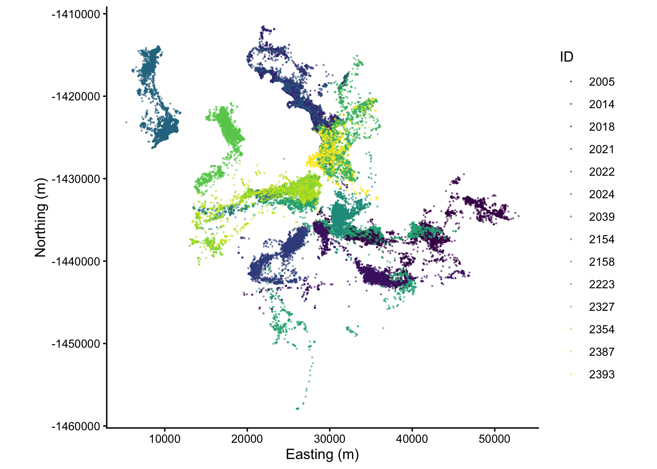
#| fig-cap: "All 14 buffalo in the dataset."
buffalo_all %>%
  ggplot(aes(x = x_, y = y_, colour = factor(id))) +
  geom_point(alpha = 0.5, size = 0.1) +
  coord_fixed() +
  scale_x_continuous("Easting (m)") +
  scale_y_continuous("Northing (m)") +
  scale_colour_viridis_d("ID") +
  theme_classic()
```
## Select a single individual and a single season
We restrict the analysis to **one individual over one season**, for two reasons.
*One individual* keeps the walkthrough focused on the simulation pipeline rather than on the modelling questions that arise with multiple animals (pooling, random effects, two-step estimation). It also makes validation unambiguous: we compare predicted space use against *this animal's* observed locations.
*One season*: Restricting to roughly the 2018 dry season keeps buffalo `r which_buffalo` within one contiguous area, and also matches our NDVI layer, which represents August 2018.
```{r}
#| label: select_individual
buffalo_id <- buffalo_all %>%
  filter(id == which_buffalo,
         t_ >= time_start,
         t_ <  time_end)

cat("Number of locations:", nrow(buffalo_id), "\n")
cat("Date range:", format(min(buffalo_id$t_)), "to", format(max(buffalo_id$t_)), "\n")
```
```{r}
#| label: plot_individual
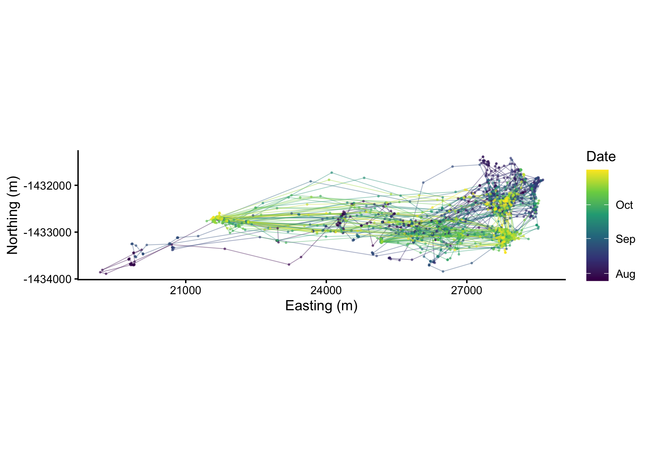
#| fig-cap: "The trajectory of the focal individual over subset period."
buffalo_id %>%
  ggplot(aes(x = x_, y = y_, colour = t_)) +
  geom_path(alpha = 0.4, linewidth = 0.3) +
  geom_point(alpha = 0.5, size = 0.3) +
  coord_fixed() +
  scale_x_continuous("Easting (m)") +
  scale_y_continuous("Northing (m)") +
  scale_colour_viridis_c("Date", trans = "time") +
  theme_classic()
```
## Check the sampling rate
Step selection analysis assumes a *regular* sampling interval. Before going further we check that assumption, because irregular fixes would make step lengths incomparable and would corrupt the mapping between step number and hour of day that the whole temporal analysis depends on.
```{r}
#| label: sampling_rate
summarize_sampling_rate(buffalo_id)
```
```{r}
#| label: plot_sampling_rate
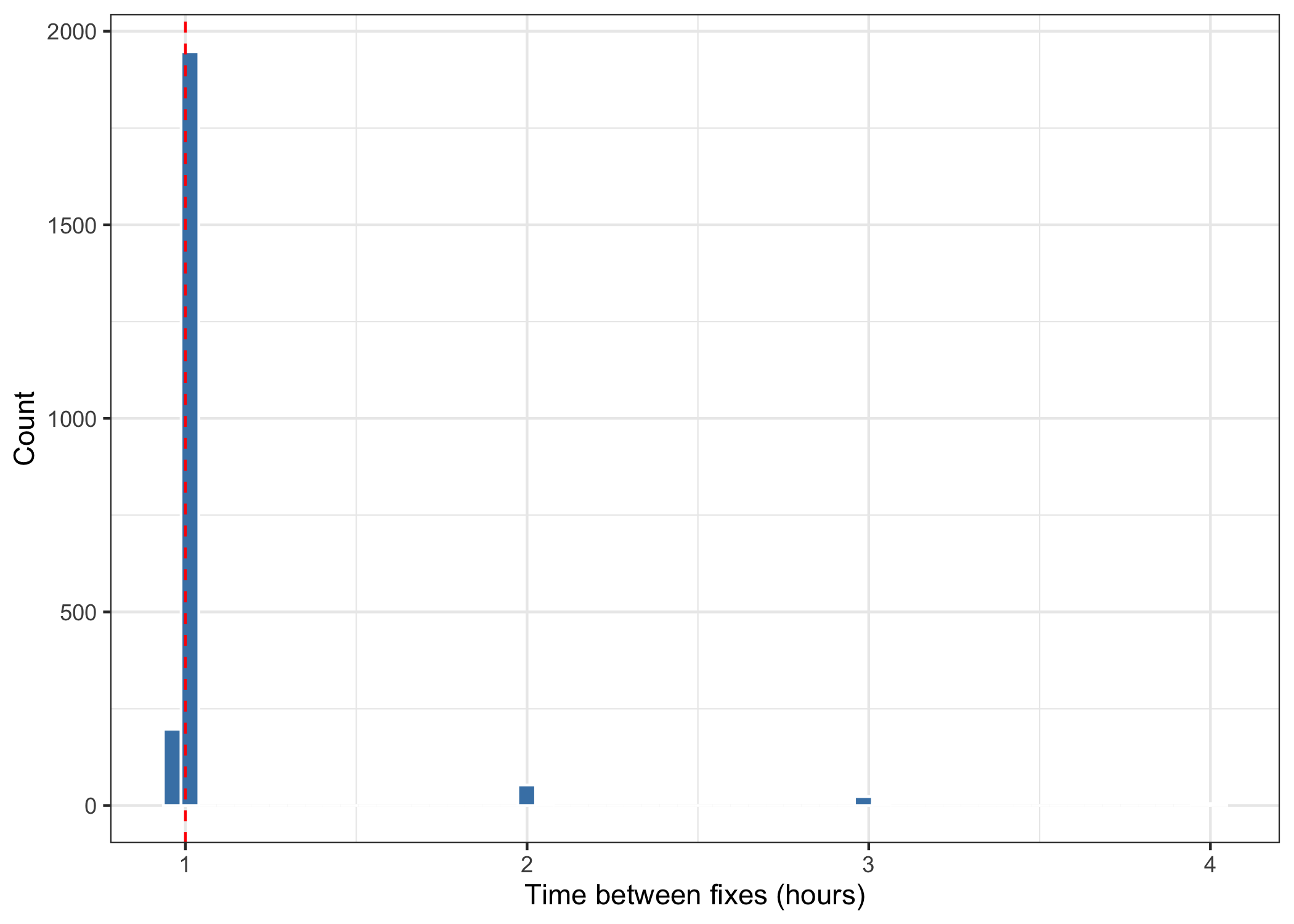
#| fig-cap: "Distribution of time intervals between consecutive fixes."
sampling_intervals <- as.numeric(diff(buffalo_id$t_), units = "hours")

ggplot(data.frame(dt = sampling_intervals[sampling_intervals < 6]), aes(x = dt)) +
  geom_histogram(bins = 60, fill = "steelblue", colour = "white") +
  geom_vline(xintercept = 1, linetype = "dashed", colour = "red") +
  labs(x = "Time between fixes (hours)", y = "Count") +
  theme_bw()
```
The majority of fixes are one hour apart, so we treat this as an hourly trajectory.
# 2. Environmental covariates
We use three covariates, all at 25 m resolution and on the same grid, which has been projected into the same GDA94 / Geoscience Australia Lambert (https://epsg.io/3112) CRS as the buffalo data.
- **NDVI** — the Normalised Difference Vegetation Index, a measure of vegetation greenness and productivity. Here it also distinguishes water bodies (strongly negative values).
- **Canopy cover** — percentage tree canopy cover, rescaled to 0–1. Relevant for shade and thermoregulation.
- **Slope** — terrain slope in degrees.
```{r}
#| label: import_rasters
ndvi <- rast("mapping/ndvi_aug_2018.tif")
names(ndvi) <- "ndvi"

# Rescale canopy cover from a percentage (0-100) to a proportion (0-1), so that
# its coefficient is on a scale comparable to the other covariates.
canopy <- rast("mapping/canopy_cover.tif") / 100
names(canopy) <- "canopy"

slope <- rast("mapping/slope_raster.tif")
names(slope) <- "slope"

# All three layers share an extent and resolution, so they can be stacked directly
covariates <- c(ndvi, canopy, slope)
covariates
```
## Define the simulation extent
Simulating over the full raster would be wasteful — most of it is far from anywhere this animal ever went, and we would need vastly more trajectories to fill it. Instead we crop to a box around the observed locations, with a generous buffer so that the simulated animal has somewhere to go.
```{r}
#| label: sim_extent
# A buffered box around the observed dry-season locations
buffer_distance <- 5000 # metres

xmin <- min(buffalo_id$x_) - buffer_distance
xmax <- max(buffalo_id$x_) + buffer_distance
ymin <- min(buffalo_id$y_) - buffer_distance
ymax <- max(buffalo_id$y_) + buffer_distance

sim_extent <- ext(xmin, xmax, ymin, ymax)

covariates_crop <- crop(covariates, sim_extent)
covariates_crop
# Individual layers, used throughout the rest of the script
ndvi_crop   <- covariates_crop[["ndvi"]]
canopy_crop <- covariates_crop[["canopy"]]
slope_crop  <- covariates_crop[["slope"]]
```
```{r}
#| label: plot_covariates
#| fig-height: 4
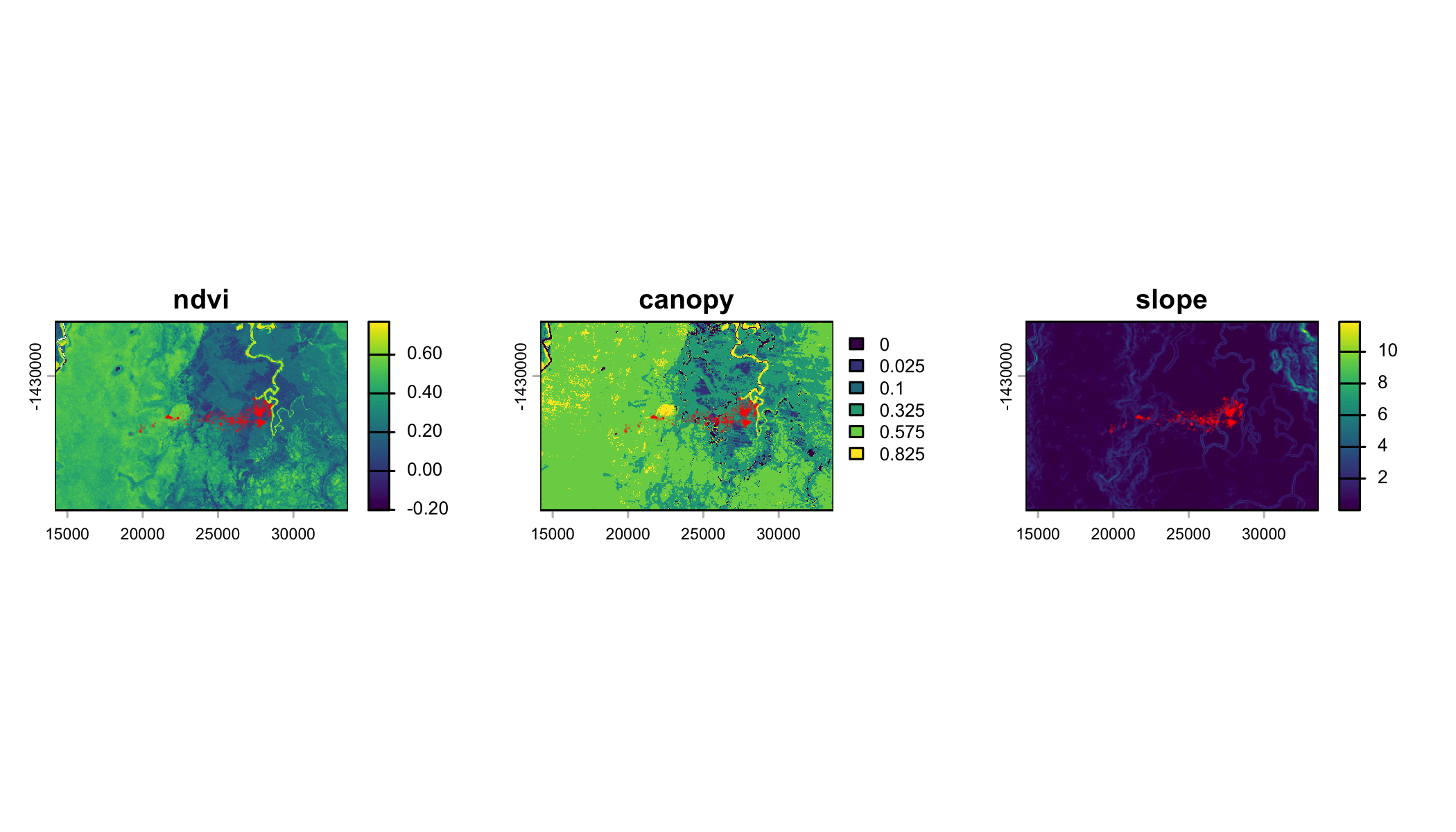
#| fig-cap: "The three covariates across the simulation extent, with observed locations in red."
par(mfrow = c(1, 3), mar = c(2, 2, 3, 4))
for (lyr in c("ndvi", "canopy", "slope")) {
  plot(covariates_crop[[lyr]], main = lyr)
  points(buffalo_id$x_, buffalo_id$y_, col = rgb(1, 0, 0, 0.15), pch = 16, cex = 0.2)
}
par(mfrow = c(1, 1))
```
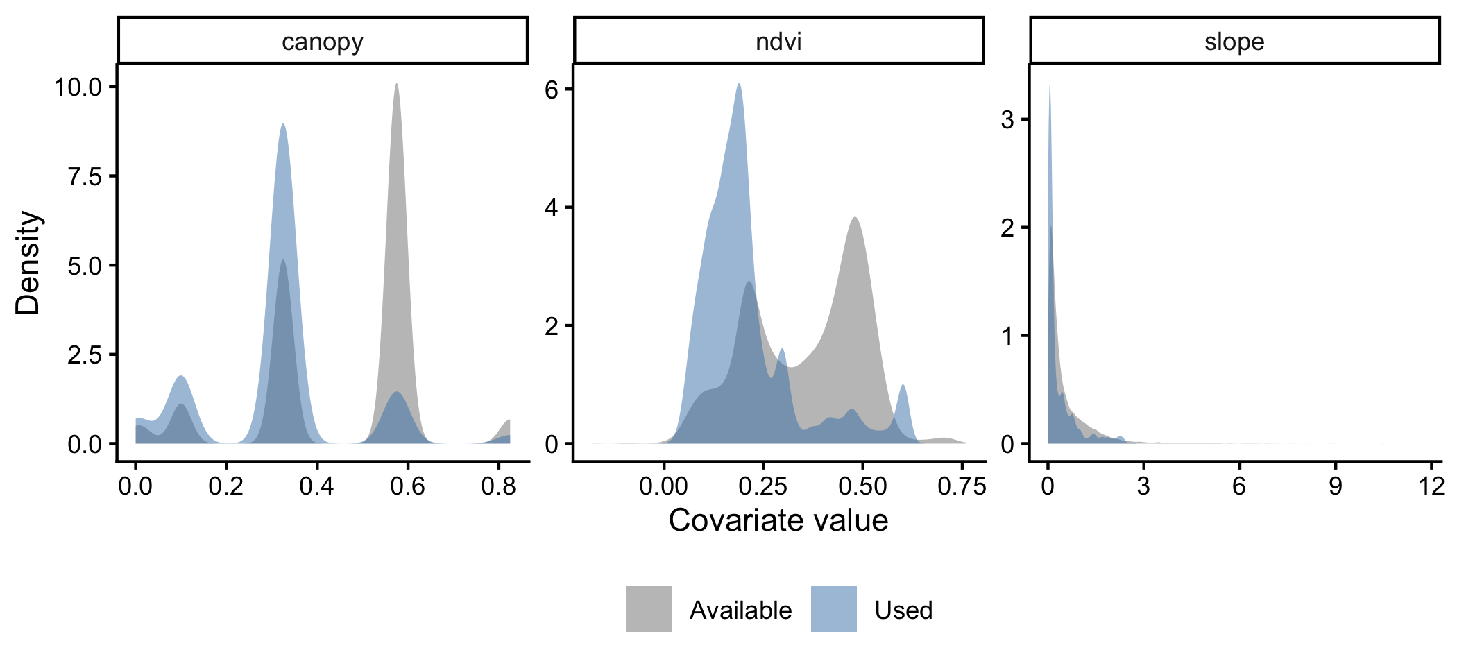
## Used versus available: across the full landscape
Before fitting anything, it is worth looking at what the animal *used* against what was *available*, for a visual assessment of (static) habitat selection. If an animal is selecting for certain habitat features, the distribution of covariate values at its locations will differ from the distribution across the landscape.
This is only a visual assessment, as it does not account for what was *available* to the animal at each step. For that, we will sample random steps to compare against the observed steps.
```{r}
#| label: used_vs_available
#| fig-height: 3.2
#| fig-cap: "Distribution of covariate values across the landscape (grey) and at observed locations (blue)."
# Covariate values at the observed locations
used_vals <- terra::extract(covariates_crop,
                            cbind(buffalo_id$x_, buffalo_id$y_)) %>%
  pivot_longer(everything(), names_to = "covariate", values_to = "value") %>%
  mutate(source = "Used")

# Covariate values across the whole landscape (a sample, for plotting speed)
avail_vals <- terra::spatSample(covariates_crop, size = 20000, na.rm = TRUE) %>%
  pivot_longer(everything(), names_to = "covariate", values_to = "value") %>%
  mutate(source = "Available")

bind_rows(avail_vals, used_vals) %>%
  filter(!is.na(value)) %>%
  ggplot(aes(x = value, fill = source)) +
  geom_density(alpha = 0.5, colour = NA) +
  facet_wrap(~ covariate, scales = "free") +
  scale_fill_manual(values = c("Available" = "grey50", "Used" = "steelblue"), name = NULL) +
  labs(x = "Covariate value", y = "Density") +
  theme_classic() +
  theme(legend.position = "bottom")
```
# 3. Generating steps and random steps
## From locations to steps
A step selection function models *steps* — the movement from one location to the next — rather than locations. Each step has a length and a turning angle relative to the previous step.
```{r}
#| label: make_steps
buffalo_steps <- buffalo_id %>% steps()

head(buffalo_steps)
```
## Tentative movement distributions
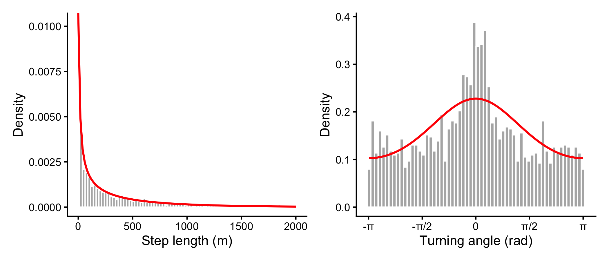
Integrated step selection analysis (iSSA) works by first fitting *tentative* distributions to the observed step lengths and turning angles, using those to generate available steps, and then **correcting** them using the coefficients that the model estimates for the movement terms [@Avgar2016-pb; @Fieberg2021-wx].
The word *tentative* is important. These are not the final estimates of the movement kernel — they are a proposal distribution. We recover the corrected parameters in section 6.
```{r}
#| label: tentative_distributions
gamma_dist    <- fit_distr(buffalo_steps$sl_, "gamma")
vonmises_dist <- fit_distr(buffalo_steps$ta_, "vonmises")

# Store the tentative parameters - we need them later for the update step
shape_tentative <- gamma_dist$params$shape
scale_tentative <- gamma_dist$params$scale
kappa_tentative <- vonmises_dist$params$kappa

cat("Tentative gamma  - shape:", round(shape_tentative, 4),
    " scale:", round(scale_tentative, 2), "\n")
cat("Tentative vonMises - kappa:", round(kappa_tentative, 4), "\n")
```
```{r}
#| label: plot_tentative
#| fig-height: 3
#| fig-cap: "Observed step lengths and turning angles with the fitted tentative distributions."
p_sl <- ggplot(buffalo_steps %>% filter(sl_ > 0), aes(x = sl_)) +
  geom_histogram(aes(y = after_stat(density)), bins = 80,
                 fill = "grey70", colour = "white") +
  stat_function(fun = dgamma,
                args = list(shape = shape_tentative, scale = scale_tentative),
                colour = "red", linewidth = 0.8) +
  scale_x_continuous("Step length (m)", limits = c(0, 2000)) +
  labs(y = "Density") +
  theme_classic()

p_ta <- ggplot(buffalo_steps %>% filter(!is.na(ta_)), aes(x = ta_)) +
  geom_histogram(aes(y = after_stat(density)), bins = 60,
                 fill = "grey70", colour = "white") +
  stat_function(fun = function(x) {
    circular::dvonmises(circular::circular(x),
                        mu = circular::circular(0), kappa = kappa_tentative)
  }, colour = "red", linewidth = 0.8) +
  scale_x_continuous("Turning angle (rad)",
                     breaks = c(-pi, -pi/2, 0, pi/2, pi),
                     labels = c("-π", "-π/2", "0", "π/2", "π")) +
  labs(y = "Density") +
  theme_classic()

p_sl + p_ta
```
## Sample available steps
For each observed (*used*) step we generate `r n_control` *available* steps from the tentative distributions, and extract the covariate values at the end of every step.
Note the naming of the movement terms: `sl_`, `log_sl_` and `cos_ta_`, each with a **trailing underscore**. This is `amt`'s convention, and following it means that `amt::update_sl_distr()` and `amt::update_ta_distr()` will work on our fitted model without any manual specification — which we make use of as a cross-check in section 6.
```{r}
#| label: random_steps
ssf_data <- buffalo_steps %>%
  random_steps(n_control = n_control,
               sl_distr  = gamma_dist,
               ta_distr  = vonmises_dist) %>%
  extract_covariates(covariates) %>%
  mutate(
    log_sl_ = log(sl_),
    cos_ta_ = cos(ta_),
    hour    = hour(t1_),   # hour of day at the START of the step
    times   = 1            # a dummy column of constant values, required by the
                           # Cox proportional hazards family in `mgcv` (see below)
  ) %>%
  # Drop steps falling outside the covariate layers, and any zero-length steps
  # (log(0) is undefined)
  filter(!is.na(ndvi), !is.na(canopy), !is.na(slope), sl_ > 0)

cat("Rows:", nrow(ssf_data),
    " | strata (used steps):", length(unique(ssf_data$step_id_)), "\n")
head(ssf_data)
```
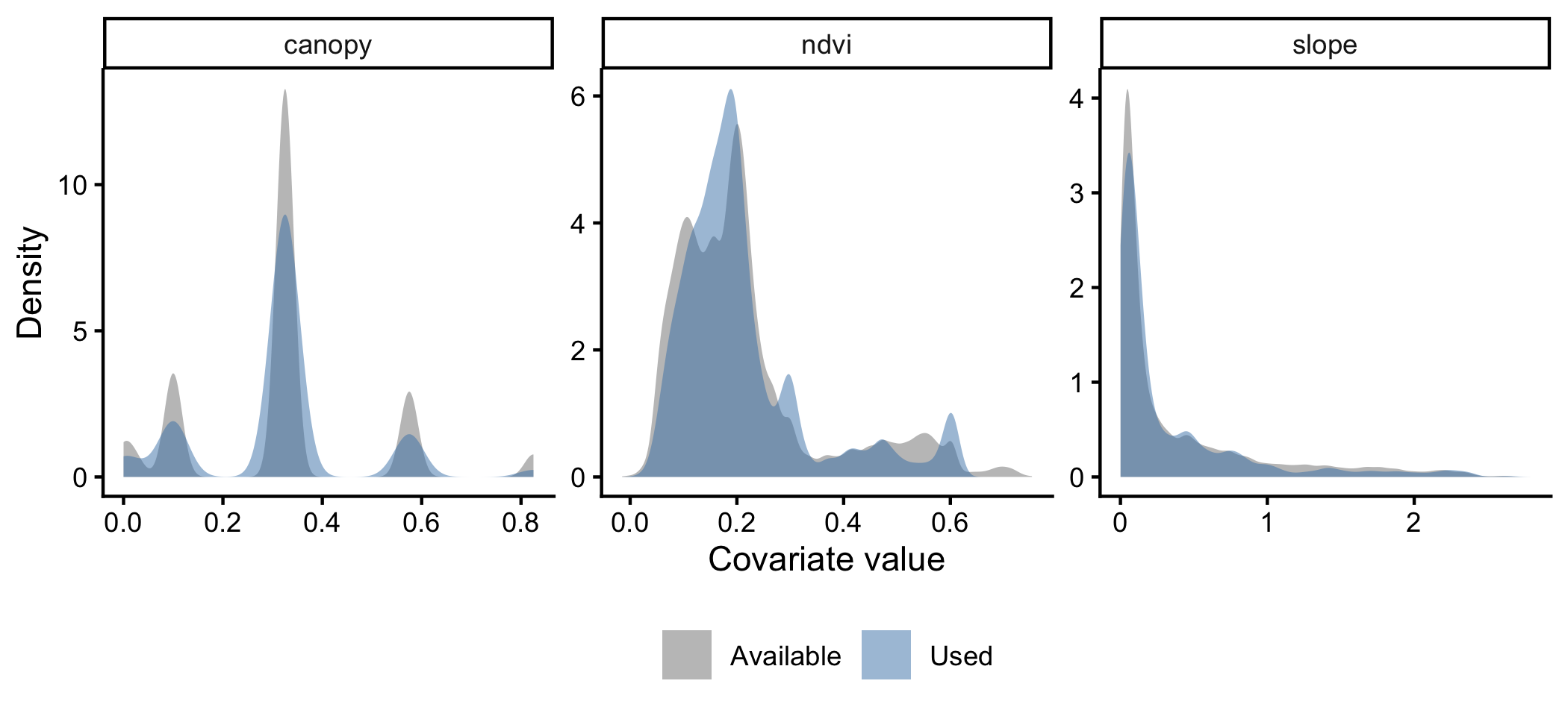
The covariate values of these *used* vs *available* steps will look more similar to one another, as the random steps are drawn from a similar region in the covariate space (to define availability), but there should still be some differences if the animal is selecting for certain habitat features.
```{r}
#| label: plot_used_available_steps
#| fig-height: 3.2
#| fig-cap: "Covariate values at the end of used steps versus available steps."
ssf_data %>%
  select(case_, ndvi, canopy, slope) %>%
  pivot_longer(c(ndvi, canopy, slope), names_to = "covariate", values_to = "value") %>%
  mutate(case_ = ifelse(case_, "Used", "Available")) %>%
  ggplot(aes(x = value, fill = case_)) +
  geom_density(alpha = 0.5, colour = NA) +
  facet_wrap(~ covariate, scales = "free") +
  scale_fill_manual(values = c("Available" = "grey50", "Used" = "steelblue"), name = NULL) +
  labs(x = "Covariate value", y = "Density") +
  theme_classic() +
  theme(legend.position = "bottom")
```
# 4. Model A — a static step selection function
## Fitting with `amt`
The standard iSSF is fitted as a conditional logistic regression, stratified by step.
```{r}
#| label: fit_static
tic("Fitting the static model with amt::fit_issf()")

ssf_static <- amt::fit_issf(
  case_ ~ ndvi + canopy + slope +      # habitat selection
    sl_ + log_sl_ + cos_ta_ +          # movement (used to correct the tentative distributions)
    strata(step_id_),                  # each used step and its available steps form a stratum
  data = ssf_data, model = TRUE)

toc()
summary(ssf_static)
```
## The same model, fitted as a GAM
We also fit the identical model using `mgcv`, via a Cox proportional hazards likelihood. A stratified Cox model with one "event" per stratum is mathematically equivalent to conditional logistic regression, so this gives the same answer — the trick is described in @Klappstein2024-ax.
Why do we fit the static model using a GAM, even though it doesn't have smooth (additive terms)? Because Model B in the next section *must* be fitted this way (we need smooth terms), and having Model A in the same framework means we can generate the prediction weights using the `predict()` function, which makes it easier to get standard errors for the predictions.
A downside is that the GAM fitting is slower than `amt::fit_issf()`, so for more complicated models and/or more data, we would probably stick to the `amt` approach unless we are fitting smooth terms.
```{r}
#| label: fit_static_gam
tic("Fitting the static model with mgcv::gam()")

ssf_static_gam <- mgcv::gam(
  cbind(times, step_id_) ~ ndvi + canopy + slope + sl_ + log_sl_ + cos_ta_,
  data = ssf_data, family = cox.ph, weight = case_)

toc()
summary(ssf_static_gam)
```
```{r}
#| label: compare_static_fits
# The two parameterisations should give the same coefficients
tibble(
  term       = names(coef(ssf_static)),
  fit_issf   = as.numeric(coef(ssf_static)),
  cox_ph_gam = as.numeric(coef(ssf_static_gam)[names(coef(ssf_static))])
) %>%
  mutate(difference = fit_issf - cox_ph_gam)
```
Both models give essentially identical results (with slight differences due to numerical precision).
## Response curves
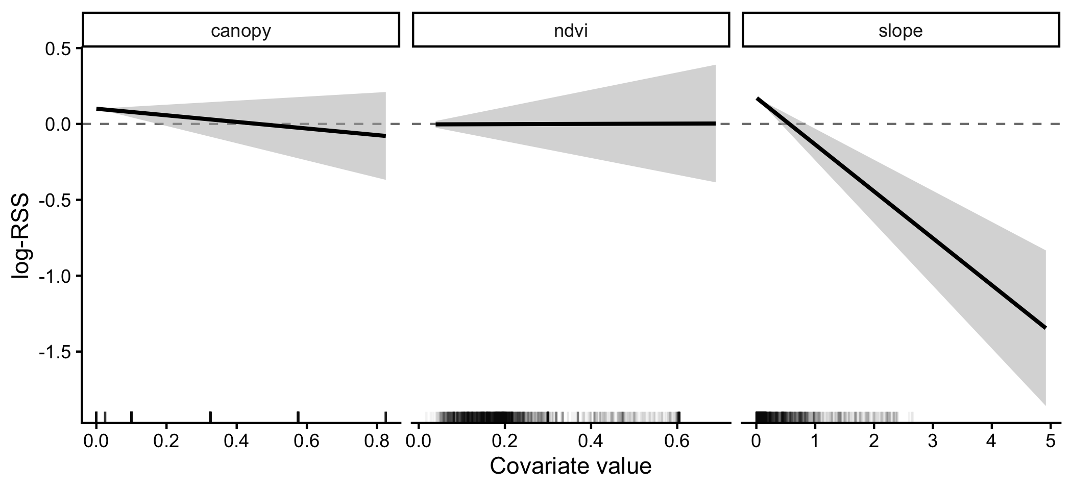
We express habitat selection as **relative selection strength** (RSS): how much more likely the animal is to select a location with a given covariate value, relative to a reference value, all else equal [@Fieberg2021-wx]. On the log scale this is just the coefficient multiplied by the covariate value.
```{r}
#| label: static_response_curves
#| fig-height: 3.2
#| fig-cap: "Log-RSS for each covariate under the static model, with 95% confidence intervals. Values are relative to the mean covariate value (dashed line at zero)."
# A sensible range of values to plot over for each covariate: the central 99%
# of the values that actually occur in the landscape.
cov_ranges <- map(c("ndvi", "canopy", "slope"), function(v) {
  q <- quantile(values(covariates_crop[[v]]), probs = c(0.005, 0.995), na.rm = TRUE)
  seq(q[1], q[2], length.out = 100)
})
names(cov_ranges) <- c("ndvi", "canopy", "slope")

# For each covariate, predict log-RSS across its range while holding the others
# at zero. Because the model is linear and has no intercept, the prediction is
# simply value * coefficient - but using predict() gives us standard errors,
# and generalises to the GAM in the next section.
static_curves <- map_dfr(names(cov_ranges), function(v) {
  nd <- data.frame(ndvi = 0, canopy = 0, slope = 0,
                   sl_ = 0, log_sl_ = 0, cos_ta_ = 0)
  nd <- nd[rep(1, length(cov_ranges[[v]])), ]
  nd[[v]] <- cov_ranges[[v]]

  p <- predict(ssf_static_gam, newdata = nd, type = "link", se.fit = TRUE)

  # Centre on the mean covariate value, so the curve reads as "relative to average"
  ref <- mean(values(covariates_crop[[v]]), na.rm = TRUE) * coef(ssf_static_gam)[[v]]

  data.frame(covariate = v,
             value     = cov_ranges[[v]],
             log_rss   = p$fit - ref,
             lower     = p$fit - ref - 1.96 * p$se.fit,
             upper     = p$fit - ref + 1.96 * p$se.fit)
})

# Observed values, for the rug
used_long <- ssf_data %>%
  filter(case_) %>%
  select(ndvi, canopy, slope) %>%
  pivot_longer(everything(), names_to = "covariate", values_to = "value")

ggplot(static_curves, aes(x = value)) +
  geom_hline(yintercept = 0, linetype = "dashed", colour = "grey50") +
  geom_ribbon(aes(ymin = lower, ymax = upper), fill = "grey70", alpha = 0.5) +
  geom_line(aes(y = log_rss), linewidth = 0.9) +
  geom_rug(data = used_long, aes(x = value), inherit.aes = FALSE,
           alpha = 0.05, sides = "b") +
  facet_wrap(~ covariate, scales = "free_x") +
  labs(x = "Covariate value", y = "log-RSS") +
  theme_classic()
```
All three coefficients are negative, so on average across the whole day this animal avoided greener, more wooded and steeper locations. But, this is *on average across the whole day*, which we change in the next model.
# 5. Model B — a temporally dynamic step selection function
## The idea
Animals do not behave the same way at 3 am as at 3 pm. A buffalo may seek shade in the heat of the day and forage in open grassland in the evening. A static model averages over all of that, producing a coefficient that may describe no hour of the day particularly well.
The fix is to let each coefficient be a *function of time of day*:
$$\omega(\mathbf{X}(s); \boldsymbol{\beta}(\tau)) = \exp\big(\beta_{1}(\tau) X_1(s) + \cdots + \beta_{n}(\tau) X_n(s)\big)$$
where $\tau$ is the hour of day. In @Forrest2025-le, we expressed each $\beta_i(\tau)$ as a sum of harmonic (sine and cosine) terms. Here we use a **cyclic penalised spline** instead, following @Klappstein2024-ax — the idea is the same, but the smoothness is chosen automatically by the model rather than by us picking a number of harmonics, and the `mgcv` and `gratia` packages contain many helpful functions for GAMs.
In `mgcv`, `s(hour, by = ndvi)` fits exactly this: a *varying-coefficient* term, in which the coefficient on `ndvi` is a smooth function of `hour`. Using `bs = "cc"` makes that function cyclic, so it joins up smoothly at midnight.
## Fitting the model
```{r}
#| label: fit_dynamic
#| cache: false
tic("Fitting the temporally dynamic model")

ssf_dynamic <- mgcv::gam(
  cbind(times, step_id_) ~
    # Habitat selection, each varying smoothly across the day
    s(hour, by = ndvi,    bs = "cc") +
    s(hour, by = canopy,  bs = "cc") +
    s(hour, by = slope,   bs = "cc") +
    # Movement, also varying across the day - this is what allows the simulated
    # animal to travel further and more directionally at some hours than others
    s(hour, by = sl_,     bs = "cc") +
    s(hour, by = log_sl_, bs = "cc") +
    s(hour, by = cos_ta_, bs = "cc"),
  # Place the cyclic knots at 0 and 24 (see the note below)
  knots  = list(hour = c(0, 24)),
  data   = ssf_data,
  family = cox.ph,
  weight = case_)

toc()
summary(ssf_dynamic)
```
## Two details worth knowing
### Why `knots = list(hour = c(0, 24))`?
Without this argument, `mgcv` places the endpoints of the cyclic basis at the *range of the data*. Our `hour` variable takes integer values 0 to 23, so the endpoints would be placed at 0 and 23 — wrapping hour 23 onto hour 0, and squeezing an hour out of the daily cycle. We can see this directly in the knot locations:
```{r}
#| label: knots_demonstration
demo <- data.frame(hour = 0:23, z = 1)

# Cyclic basis with the knots left to their default
smoothCon(s(hour, bs = "cc", k = 6), data = demo, absorb.cons = TRUE)[[1]]$xp
# Cyclic basis with the knots set explicitly
smoothCon(s(hour, bs = "cc", k = 6), data = demo,
          knots = list(hour = c(0, 24)), absorb.cons = TRUE)[[1]]$xp
```
The second is what we want: the cycle spans a full 24 hours.
## Model comparison
```{r}
#| label: model_comparison
tibble(
  model = c("A: static", "B: temporally dynamic"),
  AIC   = c(AIC(ssf_static_gam), AIC(ssf_dynamic)),
  edf   = c(sum(ssf_static_gam$edf), sum(ssf_dynamic$edf))
) %>%
  mutate(delta_AIC = AIC - min(AIC))
```
The dynamic model is overwhelmingly preferred. That is a statement` about *fit*, though — not necessarily whether it produces more accurate predictions.
## Model diagnostics
```{r}
#| label: gam_draw
#| fig-height: 6
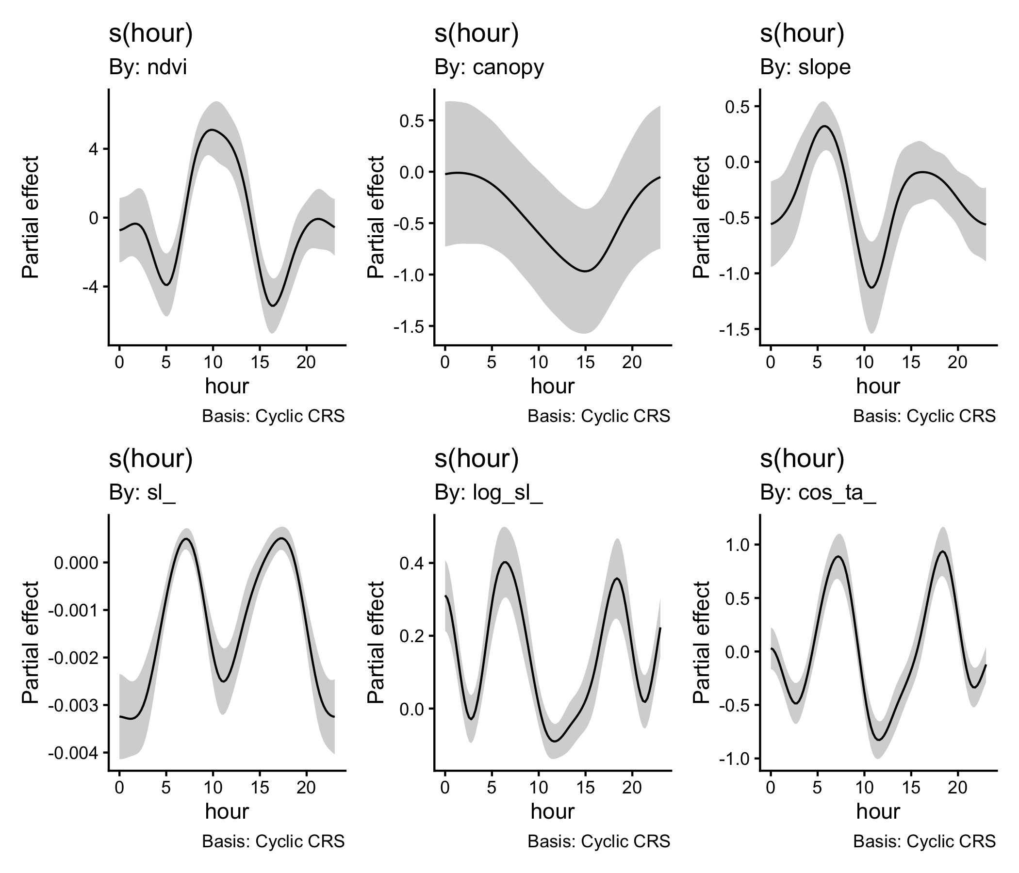
#| fig-cap: "The six estimated smooth functions. Each panel shows how the coefficient on that term varies across the day."
gratia::draw(ssf_dynamic, rug = FALSE) &
  theme_classic()
```
# 6. From fitted models to hourly coefficients
This step could be simplified if only using a static model, but as we have the temporally dynamic model, we put them both into the same format so they can be simulated from using the same process.
We reduce **each** model to the same object: a 24-row table with one row per hour of the day, and columns for the three habitat coefficients plus the three movement parameters. Model A's table has identical values in every row; Model B's cycles according to the coefficients. Everything downstream then works for either model without modification.
## Extracting habitat coefficients
Because neither model has an intercept, the prediction for `ndvi = 1`, and everything else set to 0, is $\beta_{\text{NDVI}}(\tau)$. We can set therefore set each coefficient to 1 in turn. The same call works for the static model (giving a constant for each hour) and the dynamic one (giving the smooth), and `se.fit = TRUE` gives us confidence intervals for free.
```{r}
#| label: beta_extraction_function
#' Extract the coefficient on one covariate, for each hour of the day
#'
#' @param model  a fitted `mgcv` model with no intercept
#' @param var    name of the covariate whose coefficient we want
#' @param hours  hours at which to evaluate
#' @return a data frame of hour, estimate, standard error and 95% CI
beta_by_hour <- function(model, var, hours = 0:23) {

  # A design where every covariate is zero except the one of interest, which is 1.
  # The linear predictor then equals the coefficient on that covariate.
  nd <- data.frame(hour = hours, ndvi = 0, canopy = 0, slope = 0,
                   sl_ = 0, log_sl_ = 0, cos_ta_ = 0)

  # change the variable of interest to 1
  nd[[var]] <- 1

  p <- predict(model, newdata = nd, type = "link", se.fit = TRUE)

  data.frame(hour     = hours,
             variable = var,
             estimate = as.numeric(p$fit),
             se       = as.numeric(p$se.fit)) %>%
    mutate(lower = estimate - 1.96 * se,
           upper = estimate + 1.96 * se)
}
```
We map the function over all of the covariates, and combine the results into a single data frame.
```{r}
#| label: extract_betas
model_terms <- c("ndvi", "canopy", "slope", "sl_", "log_sl_", "cos_ta_")

# static model
betas_static  <- map_dfr(model_terms, ~ beta_by_hour(ssf_static_gam, .x)) %>%
  mutate(model = "A: static")
head(betas_static)
# dynamic model
betas_dynamic <- map_dfr(model_terms, ~ beta_by_hour(ssf_dynamic, .x)) %>%
  mutate(model = "B: temporally dynamic")
head(betas_dynamic)
betas_all <- bind_rows(betas_static, betas_dynamic)
```
```{r}
#| label: plot_betas
#| fig-height: 5
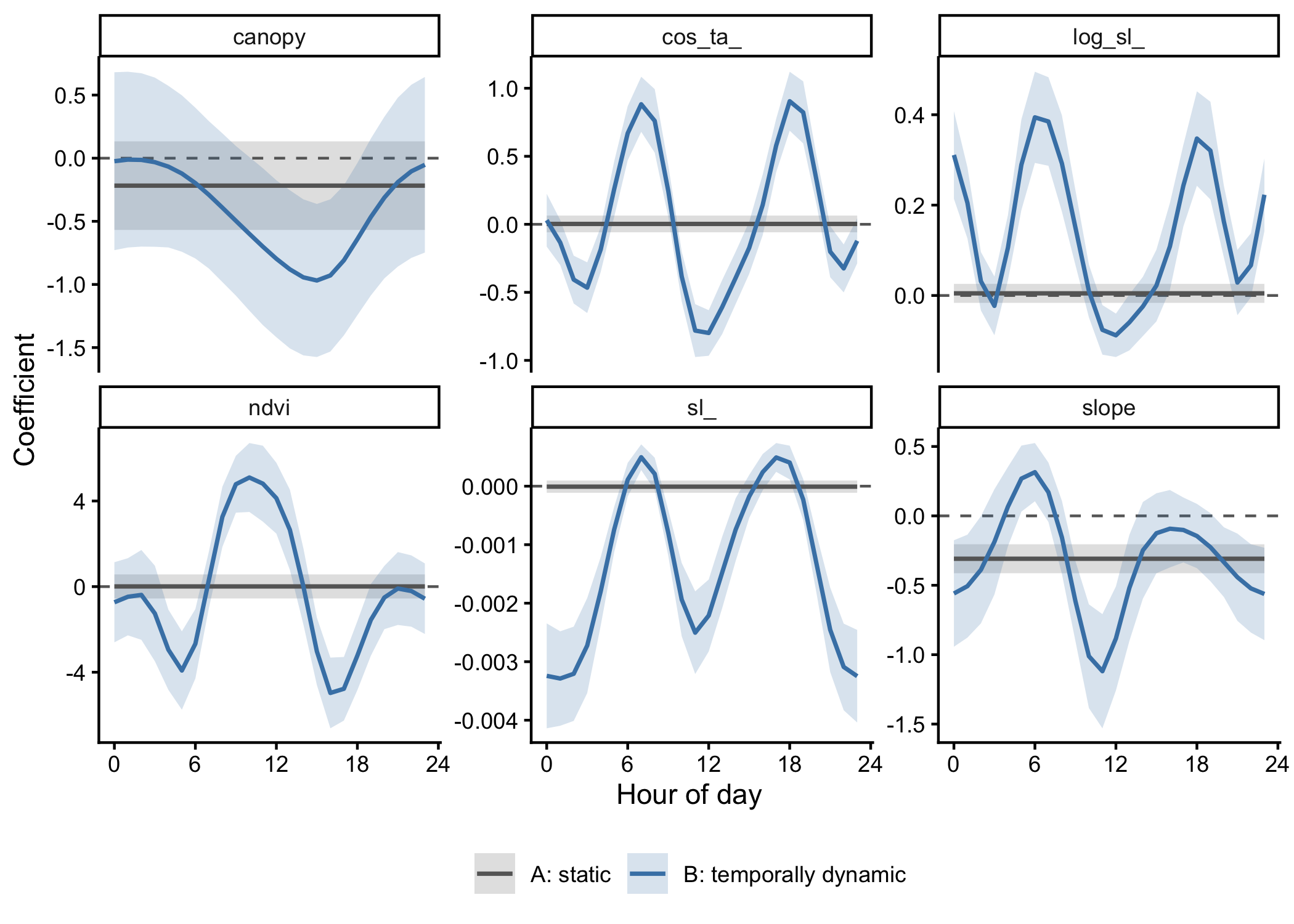
#| fig-cap: "Estimated coefficients across the day. The static model (grey) is constant by construction; the dynamic model (blue) varies."
ggplot(betas_all, aes(x = hour, y = estimate, colour = model, fill = model)) +
  geom_hline(yintercept = 0, linetype = "dashed", colour = "grey40") +
  geom_ribbon(aes(ymin = lower, ymax = upper), alpha = 0.2, colour = NA) +
  geom_line(linewidth = 0.8) +
  facet_wrap(~ variable, scales = "free_y") +
  scale_colour_manual(values = c("A: static" = "grey40",
                                 "B: temporally dynamic" = "steelblue"), name = NULL) +
  scale_fill_manual(values = c("A: static" = "grey40",
                               "B: temporally dynamic" = "steelblue"), name = NULL) +
  scale_x_continuous("Hour of day", breaks = seq(0, 24, 6)) +
  labs(y = "Coefficient") +
  theme_classic() +
  theme(legend.position = "bottom")
```
The static model's NDVI coefficient is a slightly negative constant. The dynamic model shows that this average conceals a strong daily cycle: the animal *selects* for high NDVI around the middle of the day and *avoids* it in the late afternoon and evening. Averaging those two opposite behaviours together produces a number that describes neither.
## Correcting the movement parameters
The movement coefficients are not selection coefficients — they are *corrections* to the tentative distributions we fitted in section 3. The update rules for a gamma step-length distribution and a von Mises turning-angle distribution are [@Avgar2016-pb; @Fieberg2021-wx; @Klappstein2023-ov; @Klappstein2024-ax]:
$$\text{shape}(\tau) = \text{shape}_{\text{tentative}} + \beta_{\log(\text{sl})}(\tau)$$
$$\text{scale}(\tau) = \frac{1}{\ \dfrac{1}{\text{scale}_{\text{tentative}}} - \beta_{\text{sl}}(\tau)\ }$$
$$\kappa(\tau) = \kappa_{\text{tentative}} + \beta_{\cos(\text{ta})}(\tau)$$
```{r}
#| label: build_hourly_coefs
#' Build a 24-row table of hourly coefficients and movement parameters
build_hourly_coefs <- function(model) {

  betas <- map_dfr(model_terms, ~ beta_by_hour(model, .x)) %>%
    select(hour, variable, estimate) %>%
    pivot_wider(names_from = variable, values_from = estimate)

  betas %>%
    mutate(
      # Apply the iSSA update rules to recover the corrected movement kernel
      shape = shape_tentative + log_sl_,
      scale = 1 / ((1 / scale_tentative) - sl_),
      kappa = kappa_tentative + cos_ta_
    ) %>%
    select(hour, ndvi, canopy, slope, shape, scale, kappa)
}

hourly_coefs_static  <- build_hourly_coefs(ssf_static_gam)
hourly_coefs_dynamic <- build_hourly_coefs(ssf_dynamic)

# show the dynamic model's hourly coefficients and movement parameters
hourly_coefs_dynamic
```
## Checking the update rules against `amt`
These update rules are the single most important piece of arithmetic in the script: if they are wrong, every simulated step length is wrong and nothing downstream means anything. `amt` implements them directly, so for the static model we can check our hand-computed values against the package.
```{r}
#| label: check_update_rules
amt_sl <- amt::update_sl_distr(ssf_static)
amt_ta <- amt::update_ta_distr(ssf_static)

tibble(
  parameter = c("shape", "scale", "kappa"),
  manual    = c(hourly_coefs_static$shape[1],
                hourly_coefs_static$scale[1],
                hourly_coefs_static$kappa[1]),
  amt       = c(amt_sl$params$shape, amt_sl$params$scale, amt_ta$params$kappa)
) %>%
  mutate(difference = manual - amt)
```
```{r}
#| label: plot_movement_params
#| fig-height: 3.2
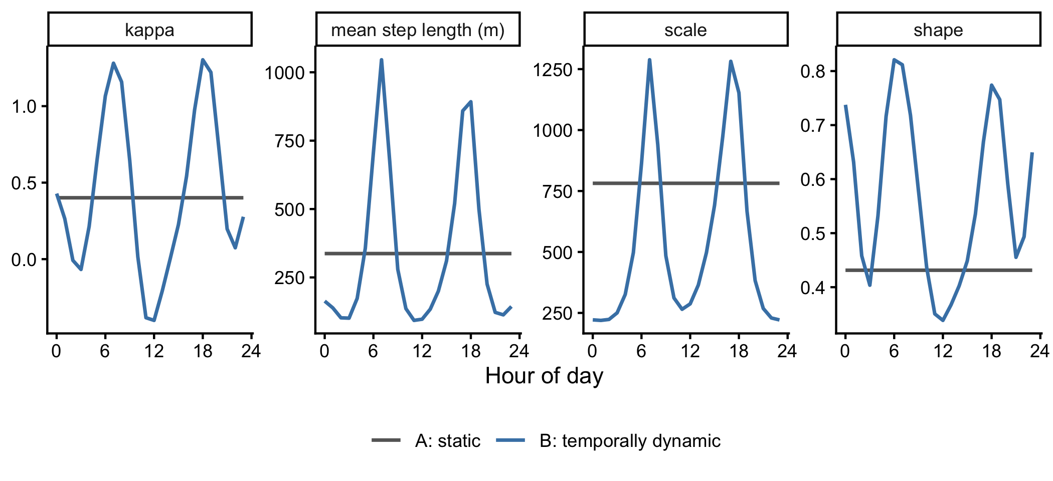
#| fig-cap: "Corrected movement parameters across the day. Mean step length is the product of shape and scale."
bind_rows(
  hourly_coefs_static  %>% mutate(model = "A: static"),
  hourly_coefs_dynamic %>% mutate(model = "B: temporally dynamic")
) %>%
  mutate(`mean step length (m)` = shape * scale) %>%
  select(hour, model, shape, scale, kappa, `mean step length (m)`) %>%
  pivot_longer(c(shape, scale, kappa, `mean step length (m)`),
               names_to = "parameter", values_to = "value") %>%
  ggplot(aes(x = hour, y = value, colour = model)) +
  geom_line(linewidth = 0.8) +
  facet_wrap(~ parameter, scales = "free_y", nrow = 1) +
  scale_colour_manual(values = c("A: static" = "grey40",
                                 "B: temporally dynamic" = "steelblue"), name = NULL) +
  scale_x_continuous("Hour of day", breaks = seq(0, 24, 6)) +
  labs(y = NULL) +
  theme_classic() +
  theme(legend.position = "bottom")
```
The dynamic model recovers a clear daily activity cycle: short steps through the middle of the day (resting) and long, directed steps in the early evening. The static model, by construction, has the animal moving the same way at every hour.
::: callout-note
## Check that the corrected parameters are valid
The update rules involve a subtraction, so it is possible in principle for them to produce an invalid distribution — a negative shape, or a negative scale if $\beta_{\text{sl}}(\tau) > 1/\text{scale}_{\text{tentative}}$. It is worth checking explicitly before simulating, rather than discovering it as an obscure error inside the simulation loop. A negative kappa is valid, but it means the animal is turning *away* from its previous direction rather than towards it, so we check the range of kappa as well.
:::
```{r}
#| label: validate_movement_params
hourly_coefs_dynamic %>%
  summarise(
    min_shape       = min(shape),
    min_scale       = min(scale),
    shape_all_valid = all(shape > 0),
    scale_all_valid = all(scale > 0),
    kappa_range     = paste(round(range(kappa), 3), collapse = " to ")
  )
```
# 7. Pre-computing hourly habitat selection surfaces
For the simulation we need, at every candidate step, the value of the habitat selection function
$$\log \omega(\mathbf{X}(s); \boldsymbol{\beta}(\tau)) = \beta_{\text{NDVI}}(\tau)\,\text{NDVI}(s) + \beta_{\text{canopy}}(\tau)\,\text{canopy}(s) + \beta_{\text{slope}}(\tau)\,\text{slope}(s)$$
Rather than evaluating this at each of the millions of candidate steps we will generate, we compute it **once per hour** across the whole landscape, producing a 24-layer raster stack. The simulation then just looks up a value. We keep everything on the log scale and exponentiate only when sampling, which is both faster and numerically safer.
```{r}
#| label: rsf_surfaces
#' Build a 24-layer raster stack of log habitat selection values, one per hour
build_hourly_surfaces <- function(hourly_coefs) {

  layers <- map(1:24, function(i) {
    cf <- hourly_coefs[i, ]
    # Linear predictor for this hour, across the whole landscape
    ndvi_crop * cf$ndvi + canopy_crop * cf$canopy + slope_crop * cf$slope
  })

  stk <- rast(layers)
  names(stk) <- paste0("hour_", hourly_coefs$hour)
  stk
}

tic("Building hourly selection surfaces")
surfaces_static  <- build_hourly_surfaces(hourly_coefs_static)
surfaces_dynamic <- build_hourly_surfaces(hourly_coefs_dynamic)
toc()
surfaces_dynamic
```
```{r}
#| label: plot_surfaces
#| fig-height: 6
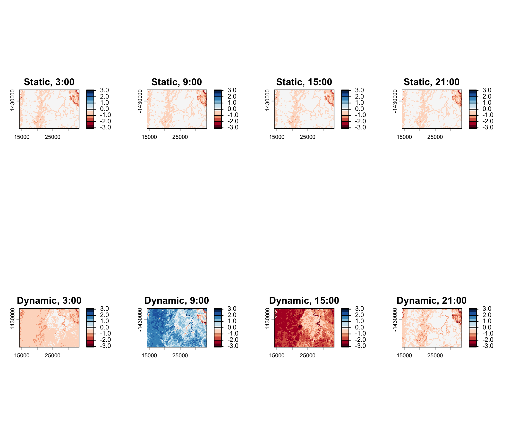
#| fig-cap: "Log habitat selection surfaces at four times of day. The static model is identical at every hour; the dynamic model changes markedly."
# A shared, symmetric colour scale so the panels are comparable
# sel_range <- range(c(values(surfaces_dynamic), values(surfaces_static)), na.rm = TRUE)
# there are some extreme outliers so we'll take the 0.5% and 99.5% quantiles instead
sel_range <- quantile(c(values(surfaces_dynamic), values(surfaces_static)), probs = c(0.005, 0.995), na.rm = TRUE)
sel_max   <- max(abs(sel_range))

plot_hours <- c(3, 9, 15, 21)

par(mfrow = c(2, 4), mar = c(2, 2, 3, 4))
for (h in plot_hours) {
  plot(surfaces_static[[h + 1]], main = paste0("Static, ", h, ":00"),
       range = c(-sel_max, sel_max), col = brewer.pal(11, "RdBu"))
}
for (h in plot_hours) {
  plot(surfaces_dynamic[[h + 1]], main = paste0("Dynamic, ", h, ":00"),
       range = c(-sel_max, sel_max), col = brewer.pal(11, "RdBu"))
}
par(mfrow = c(1, 1))
```
## An animation of the daily cycle
The daily cycle is much easier to appreciate as an animation than as four static panels.
```{r}
#| label: surfaces_gif
#| results: hide
surface_gif_path <- file.path(figure_save_path, "hourly_selection_surfaces.gif")

# Render one frame per hour, all on the same colour scale so that the animation
# shows genuine change rather than rescaling
frame_files <- map_chr(0:23, function(h) {
  f <- file.path(plot_save_path, sprintf("surface_frame_%02d.png", h))
  png(f, width = 150, height = 150, units = "mm", res = 150)
  plot(surfaces_dynamic[[h + 1]],
       main = sprintf("Habitat selection, %02d:00", h),
       range = c(-sel_max, sel_max), col = brewer.pal(11, "RdBu"))
  dev.off()
  f
})

image_read(frame_files) %>%
  image_animate(fps = 4) %>%
  image_write(surface_gif_path)

# Tidy up the individual frames
unlink(frame_files)
```
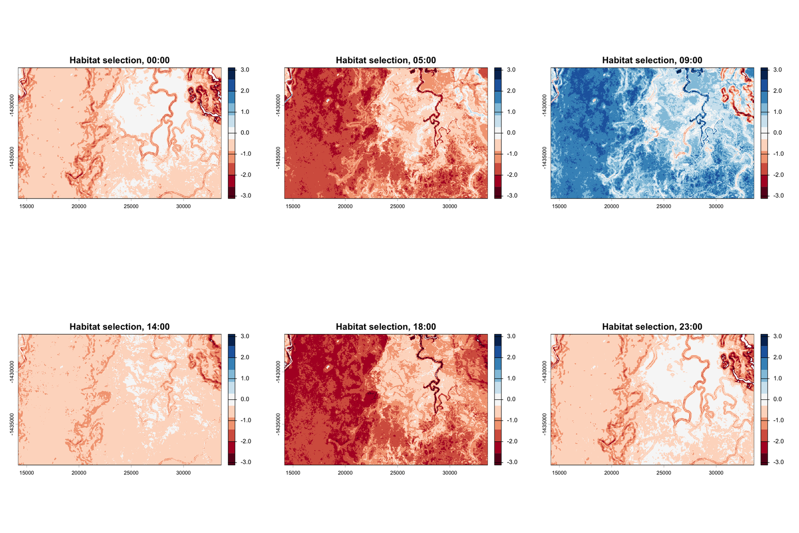
# 8. Simulating trajectories
## The redistribution kernel
Simulating from a fitted SSF means repeatedly sampling the next location from a **redistribution kernel**, which is the product of two parts:
$$\underbrace{\phi(s' \mid s, \tau)}_{\text{movement kernel}} \times \underbrace{\omega(\mathbf{X}(s'); \boldsymbol{\beta}(\tau))}_{\text{habitat kernel}}$$
In practice we approximate this by sampling: propose `r n_ch` candidate steps from the movement kernel, weight each by its habitat value, and choose one with probability proportional to that weight. This is exactly the structure of the model we fitted.
## A fast raster lookup
The simulation needs tens of millions of raster lookups. `terra::extract()` is convenient but carries a per-call overhead that creates a bottleneck when it is called hundreds of thousands of times, so we extract the raster values into a plain matrix once, and index into it with arithmetic.
```{r}
#| label: fast_extract
#' Pre-digest a raster stack into a plain matrix plus its geometry
#'
#' `terra::values()` returns a matrix with one row per cell (in row-major order)
#' and one column per layer, which is exactly what we need for fast indexing.
prepare_lookup <- function(cov_stack) {
  list(vals = terra::values(cov_stack),
       xmin = xmin(cov_stack), ymax = ymax(cov_stack),
       nrow = nrow(cov_stack), ncol = ncol(cov_stack),
       resx = res(cov_stack)[1], resy = res(cov_stack)[2])
}

#' Look up values at coordinates in a given layer
#'
#' Equivalent to `terra::extract(cov_stack[[layer]], cbind(x, y))[, 1]`, but without the
#' per-call overhead. Coordinates outside the raster return NA.
lookup <- function(lk, x, y, layer) {
  col <- floor((x - lk$xmin) / lk$resx) + 1
  row <- floor((lk$ymax - y) / lk$resy) + 1

  # `%in%`-style guard: a non-finite coordinate is not inside the raster. Without
  # `isTRUE`-style handling, a NaN coordinate would make `inside` NA rather than
  # FALSE, and NA is not permitted as a subscript in the assignment below.
  inside <- !is.na(col) & !is.na(row) &
    col >= 1 & col <= lk$ncol & row >= 1 & row <= lk$nrow

  out <- rep(NA_real_, length(x))
  cell <- (row[inside] - 1) * lk$ncol + col[inside]
  out[inside] <- lk$vals[cell, layer]
  out
}
```
```{r}
#| label: check_fast_extract
# Confirm the fast lookup agrees with terra on a sample of points
check_x <- runif(1000, xmin(surfaces_dynamic), xmax(surfaces_dynamic))
check_y <- runif(1000, ymin(surfaces_dynamic), ymax(surfaces_dynamic))

lk_check   <- prepare_lookup(surfaces_dynamic)
fast_vals  <- lookup(lk_check, check_x, check_y, 12)
terra_vals <- terra::extract(surfaces_dynamic[[12]], cbind(check_x, check_y))[, 1]

cat("Maximum absolute difference:",
    max(abs(fast_vals - terra_vals), na.rm = TRUE), "\n")
cat("NA agreement:", all(is.na(fast_vals) == is.na(terra_vals)), "\n")
```
## The simulation function
```{r}
#| label: simulate_function
#' Simulate a single trajectory from a fitted step selection function
#'
#' @param n_steps  number of steps to simulate
#' @param n_ch     number of candidate steps proposed at each step
#' @param coefs    24-row table of hourly coefficients and movement parameters
#' @param xy0      starting location, as c(x, y), on the shifted (origin at 0,0) grid
#' @param lk       lookup object from `prepare_lookup()`
#' @param boundary "wrapped" (toroidal) or "reflective"
#' @param start_hour hour of day at which the trajectory begins
#'
#' @return a data frame with one row per step
simulate_ssf <- function(n_steps, n_ch, coefs, xy0, lk,
                         boundary = "wrapped", start_hour = 0) {

  # Landscape dimensions, used for the wrapped boundary
  x_extent <- lk$ncol * lk$resx
  y_extent <- lk$nrow * lk$resy

  # --- Pre-draw all the random numbers -----------------------------------
  # Drawing all step lengths and turning angles up front is far faster than
  # drawing them one step at a time inside the loop.

  # Which hour each step occurs in (1-24, indexing into `coefs`)
  step_hours <- ((start_hour + seq_len(n_steps) - 1) %% 24) + 1

  # Step lengths: gamma, with hour-specific shape and scale
  sl <- rgamma(n_steps * n_ch,
               shape = rep(coefs$shape[step_hours], each = n_ch),
               scale = rep(coefs$scale[step_hours], each = n_ch))

  # Turning angles: von Mises, with hour-specific concentration.
  # A positive kappa means directional persistence (angles concentrated around 0),
  # a negative kappa means a tendency to reverse (angles concentrated around pi).
  # `rvonmises` returns angles on [0, 2*pi), so we draw around `mu` and subtract
  # pi to get angles on [-pi, pi).
  #
  # Only 24 distinct concentrations occur, so rather than drawing step by step we
  # draw all the angles for each hour in one call and scatter them into position.
  # `outer()` builds the destination indices: for step i the candidates occupy
  # positions ((i - 1) * n_ch + 1) to (i * n_ch).
  ta <- numeric(n_steps * n_ch)
  for (h in unique(step_hours)) {
    steps_h <- which(step_hours == h)
    kappa_h <- coefs$kappa[h]
    mu_h    <- if (kappa_h > 0) pi else 0

    ta[as.vector(outer(seq_len(n_ch), (steps_h - 1) * n_ch, "+"))] <-
      as.numeric(circular::rvonmises(n     = length(steps_h) * n_ch,
                                     mu    = circular::circular(mu_h),
                                     kappa = abs(kappa_h))) - pi
  }

  # --- Storage ------------------------------------------------------------
  x <- y <- step_length <- angle <- bearing <- hab_p <- rep(NA_real_, n_steps)

  x[1] <- xy0[1]
  y[1] <- xy0[2]
  step_length[1] <- 0
  angle[1]   <- 0
  bearing[1] <- runif(1, -pi, pi)   # arbitrary initial heading
  hab_p[1]   <- 0

  # --- The main loop ------------------------------------------------------
  for (i in 2:n_steps) {

    idx <- ((i - 1) * n_ch + 1):(i * n_ch)   # this step's candidate draws

    sl_prop <- sl[idx]
    ta_prop <- ta[idx]

    # Project the candidate endpoints from the current location. The new bearing
    # is the previous bearing plus the turning angle.
    bearing_prop <- bearing[i - 1] + ta_prop
    x_prop <- x[i - 1] + sl_prop * cos(bearing_prop)
    y_prop <- y[i - 1] + sl_prop * sin(bearing_prop)

    if (boundary == "wrapped") {
      # A toroidal landscape: an animal leaving one edge re-enters at the
      # opposite one. This removes edge effects, so the simulated process has a
      # well-defined stationary distribution. Requires the origin at (0, 0),
      # which is why we shift the rasters before simulating.
      x_prop <- x_prop %% x_extent
      y_prop <- y_prop %% y_extent
    }
    # For a reflective boundary we do nothing here: candidates outside the
    # landscape return NA from the lookup and are given negligible weight below.

    # Habitat selection value at each candidate endpoint, for this hour
    hour_layer <- step_hours[i]
    p <- lookup(lk, x_prop, y_prop, hour_layer)

    # Candidates outside the landscape (or on missing data) get a very low
    # weight rather than being dropped, so that the sample size stays constant
    p[is.na(p)] <- -50

    # Choose one candidate, with probability proportional to its habitat value.
    # This is the sampling approximation to the redistribution kernel.
    w <- sample.int(n_ch, size = 1, prob = exp(p))

    x[i] <- x_prop[w]
    y[i] <- y_prop[w]
    step_length[i] <- sl_prop[w]
    angle[i]   <- ta_prop[w]
    bearing[i] <- bearing_prop[w]
    hab_p[i]   <- p[w]
  }

  data.frame(step = seq_len(n_steps),
             hour = (step_hours - 1),
             x = x, y = y,
             sl = step_length, ta = angle, bearing = bearing,
             hab_p = hab_p)
}
```
::: callout-warning
## A note on `Rfast::rvonmises`
The code in `dynamic_SSF_sims` draws turning angles with `Rfast::rvonmises()`. Two problems showed up once the simulation was run at scale, both worth knowing about if you are adapting that code:
- **It does not respect `set.seed()`.** `Rfast` uses its own random number generator, so the simulations are not reproducible no matter what seed you set.
- **It very occasionally returns `NaN`**: about 1 draw in 8 million, at small positive concentrations. That sounds negligible until you count the draws. At `r n_traj` × `r n_steps` × `r n_ch` we make around 9 million per model, so roughly one `NaN` per run — enough that it stops the simulations.
`circular::rvonmises()` is reproducible, produced no non-finite values in 4.8 × 10⁷ draws with these parameters, and is slightly faster, so that is what we use.
:::
## Shifting the origin
The wrapped boundary uses the modulo operator, which requires the landscape origin to be at $(0,0)$. We shift the rasters accordingly, and remember the offset so we can shift the simulated coordinates back afterwards.
```{r}
#| label: shift_origin
# Remember the true extent
x_offset <- xmin(surfaces_dynamic)
y_offset <- ymin(surfaces_dynamic)

shift_to_origin <- function(stk) {
  shifted <- stk
  ext(shifted) <- c(0, xmax(stk) - xmin(stk), 0, ymax(stk) - ymin(stk))
  shifted
}

surfaces_static_shifted  <- shift_to_origin(surfaces_static)
surfaces_dynamic_shifted <- shift_to_origin(surfaces_dynamic)

lookup_static  <- prepare_lookup(surfaces_static_shifted)
lookup_dynamic <- prepare_lookup(surfaces_dynamic_shifted)
```
## Choosing starting locations
Depending on the goal of the predictions, you might want to start the simulations from different starting locations.
### Observed
If we were replicating a single animal's behaviour, such as for *animal-centric* questions like how many times a road was crossed, we might want to start every trajectory at the animal's actual location at the beginning of the period, and run for the same number of steps. This is what the `observed` option does. If you are using this option, you might want to set the number of **burn-in steps** to be 0.
### Observed sample
Similar to the approach above, except that the starting locations are drawn from **any** of the observed data. You might use this if you want to start the simulations in the same general area the animal actually used, but not all from a single point.
### Random
If you are interested in the *landscape-centric* predictions like utilisation distributions or landscape connectivity, our predictions are typically independent of where the animals start. We therefore seed the simulations uniformly across the landscape, so that they explore all available habitat rather than being biased towards a single starting point. If there are features that are inaccessible, such as water, you may want an additional mask to resample or remove those starting locations.
```{r}
#| label: start_locations
#' Generate starting locations for simulated trajectories
#'
#' @param mode one of "observed", "observed_sample" or "random"
#' @param n    number of starting locations required
#' @return an n x 2 matrix of coordinates on the shifted grid
make_start_locations <- function(mode, n) {

  if (mode == "observed") {
    # Every trajectory starts where the animal actually was at the beginning of
    # the period. Asks: "where would this animal have gone from where it was?"
    # The emergent pattern is home-range-like. Appropriate for short simulations
    # and for questions about individual space use.
    first_loc <- buffalo_id[1, ]
    matrix(rep(c(first_loc$x_ - x_offset, first_loc$y_ - y_offset), each = n),
           ncol = 2)

  } else if (mode == "observed_sample") {
    # Starts drawn from the observed locations: seeded in habitat the animal
    # genuinely used, but not all from a single point, so the resulting
    # distribution is not dominated by one origin.
    idx <- sample(nrow(buffalo_id), n, replace = TRUE)
    cbind(buffalo_id$x_[idx] - x_offset,
          buffalo_id$y_[idx] - y_offset)

  } else if (mode == "random") {
    # Uniform across the landscape. Asks: "what is the stationary distribution of
    # this movement process over this landscape?" This is what a long-term
    # utilisation distribution and its validation require, and it is what was
    # used in the paper.
    cbind(runif(n, 0, lookup_dynamic$ncol * lookup_dynamic$resx),
          runif(n, 0, lookup_dynamic$nrow * lookup_dynamic$resy))

  } else {
    stop("`mode` must be one of 'observed', 'observed_sample' or 'random'")
  }
}
```
::: callout-tip
## How starting location, boundary and burn-in interact
- `"random"` + `"wrapped"` + a burn-in converges to the **stationary distribution** of the movement process.
- `"observed"` + `"reflective"` keeps the trajectory anchored where the animal really was, which is what you might want for an **animal-centric** question or for plotting illustrative paths to compare against the observed data.
:::
## Running the simulations
```{r}
#| label: run_simulations
#' Run a set of trajectories and return them as a single data frame
#'
#' Each call seeds the random number generator explicitly. A single `set.seed()`
#' at the top of a document is not enough to make results like these
#' reproducible: every random draw made earlier in the script shifts the state
#' the simulation starts from, so adding a plot or changing the number of
#' available steps silently changes the simulated trajectories too. Seeding here
#' isolates each simulation set from everything upstream of it.
run_simulation_set <- function(lk, coefs, mode, n_traj, n_steps, boundary, burn_in, label,
                               seed) {

  set.seed(seed)

  starts <- make_start_locations(mode, n_traj)

  tic(paste0("Simulating: ", label))
  trajectories <- map(seq_len(n_traj), function(i) {
    simulate_ssf(n_steps  = n_steps,
                 n_ch     = n_ch,
                 coefs    = coefs,
                 xy0      = starts[i, ],
                 lk       = lk,
                 boundary = boundary,
                 start_hour = 0) %>%
      mutate(traj_id = i)
  })
  toc()

  bind_rows(trajectories) %>%
    # Discard the burn-in period
    filter(step > burn_in) %>%
    # Shift back to the true coordinate system
    mutate(x = x + x_offset,
           y = y + y_offset,
           model = label)
}
```
```{r}
#| label: simulate_main
# The two main simulation sets: both models, seeded at random across the
# landscape, with a wrapped boundary. These are what we aggregate and validate.
sims_static <- run_simulation_set(
  lk = lookup_static, coefs = hourly_coefs_static, mode = "random",
  n_traj = n_traj, n_steps = n_steps, boundary = "wrapped", burn_in = burn_in,
  label = "A: static", seed = 101)
sims_dynamic <- run_simulation_set(
  lk = lookup_dynamic, coefs = hourly_coefs_dynamic, mode = "random",
  n_traj = n_traj, n_steps = n_steps, boundary = "wrapped", burn_in = burn_in,
  label = "B: temporally dynamic", seed = 102)
cat("Simulated locations - static:", nrow(sims_static),
    " dynamic:", nrow(sims_dynamic), "\n")
```
## Example trajectories
For plotting we simulate some additional trajectories with a reflective boundary, just so that paths do not jump across the frame.
```{r}
#| label: example_trajectories
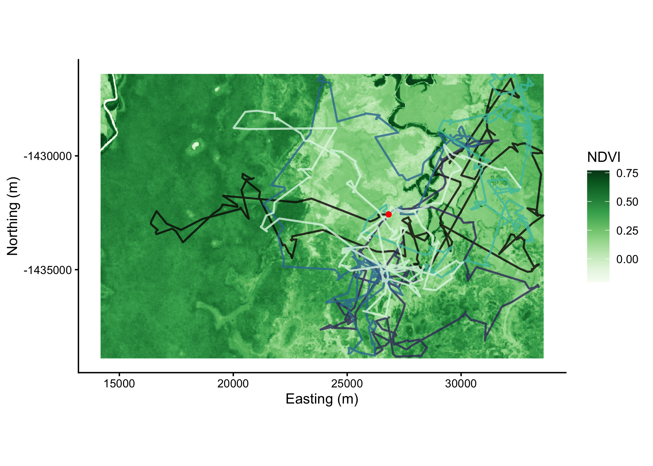
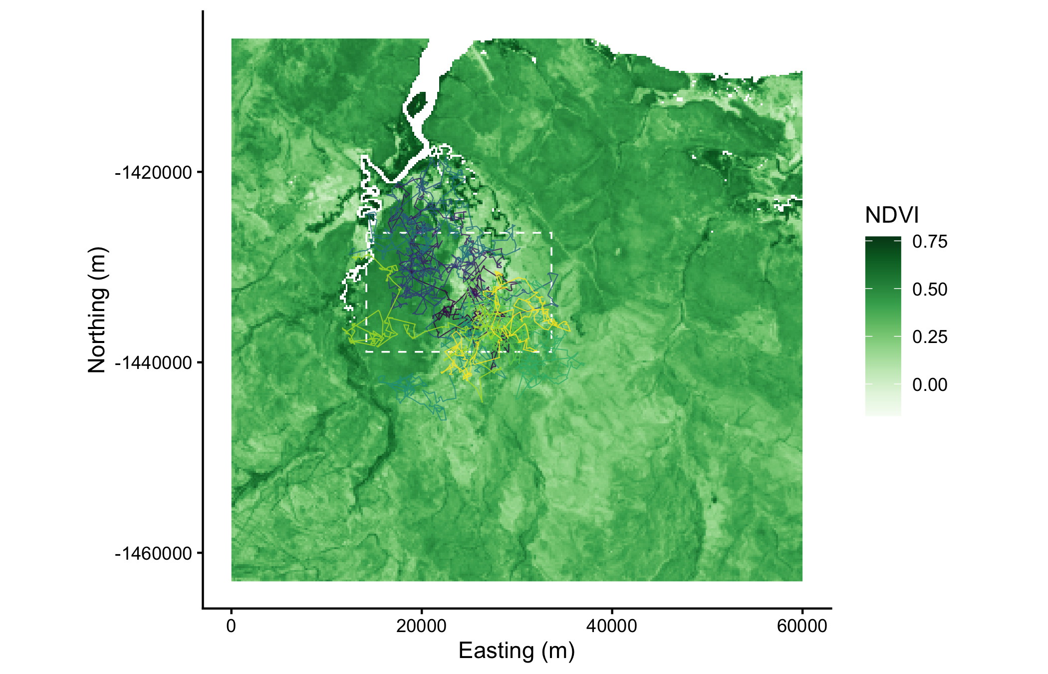
#| fig-cap: "Five example simulated trajectories from the dynamic model, over the NDVI layer."
example_trajs <- run_simulation_set(
  lk = lookup_dynamic, coefs = hourly_coefs_dynamic, mode = "observed",
  n_traj = 5, n_steps = 250, boundary = "reflective", burn_in = 0,
  label = "example", seed = 104)
ndvi_df <- as.data.frame(ndvi_crop, xy = TRUE)

ggplot() +
  geom_raster(data = ndvi_df, aes(x = x, y = y, fill = ndvi)) +
  geom_path(data = example_trajs,
            aes(x = x, y = y, colour = factor(traj_id)),
            alpha = 0.8, linewidth = 0.75) +
  geom_point(data = buffalo_id, aes(x = x_[1], y = y_[1]),
             colour = "red", size = 1.5, alpha = 0.5) +
  scale_fill_gradientn(colours = brewer.pal(9, "Greens"), name = "NDVI") +
  scale_colour_viridis_d("Trajectory", guide = "none", option = "G") +
  coord_equal() +
  labs(x = "Easting (m)", y = "Northing (m)") +
  theme_classic()
```
```{r}
#| label: plot_simulated_step_lengths
#| fig-height: 3
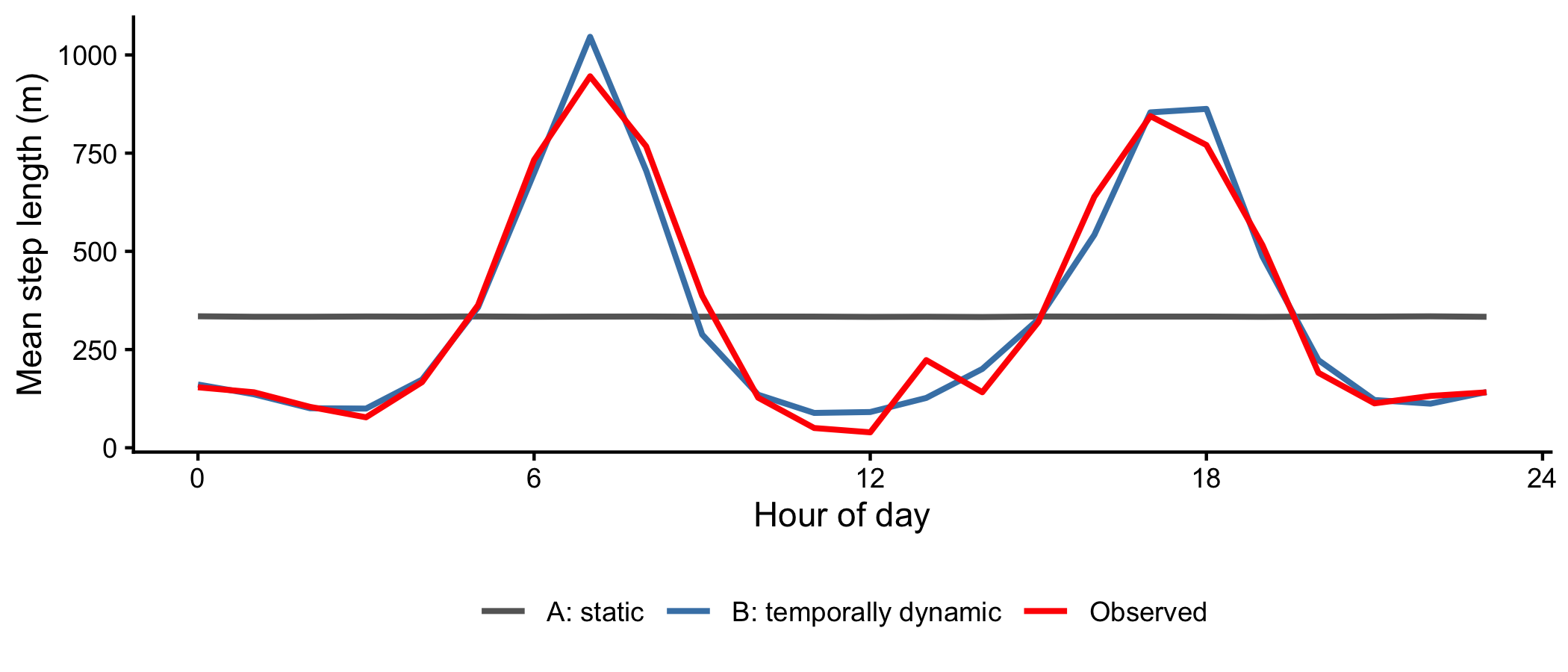
#| fig-cap: "Hourly mean step length in the simulations, compared with the observed data."
bind_rows(
  sims_static  %>% select(hour, sl, model),
  sims_dynamic %>% select(hour, sl, model)
) %>%
  group_by(model, hour) %>%
  summarise(mean_sl = mean(sl, na.rm = TRUE), .groups = "drop") %>%
  bind_rows(
    buffalo_steps %>%
      mutate(hour = hour(t1_)) %>%
      group_by(hour) %>%
      summarise(mean_sl = mean(sl_, na.rm = TRUE), .groups = "drop") %>%
      mutate(model = "Observed")
  ) %>%
  ggplot(aes(x = hour, y = mean_sl, colour = model)) +
  geom_line(linewidth = 0.9) +
  scale_colour_manual(values = c("A: static" = "grey40",
                                 "B: temporally dynamic" = "steelblue",
                                 "Observed" = "red"), name = NULL) +
  scale_x_continuous("Hour of day", breaks = seq(0, 24, 6)) +
  labs(y = "Mean step length (m)") +
  theme_classic() +
  theme(legend.position = "bottom")
```
An immediate and encouraging result: the dynamic model reproduces the observed daily activity cycle closely, while the static model — which cannot do otherwise — predicts a flat line.
# 9. Aggregating simulations into utilisation distributions
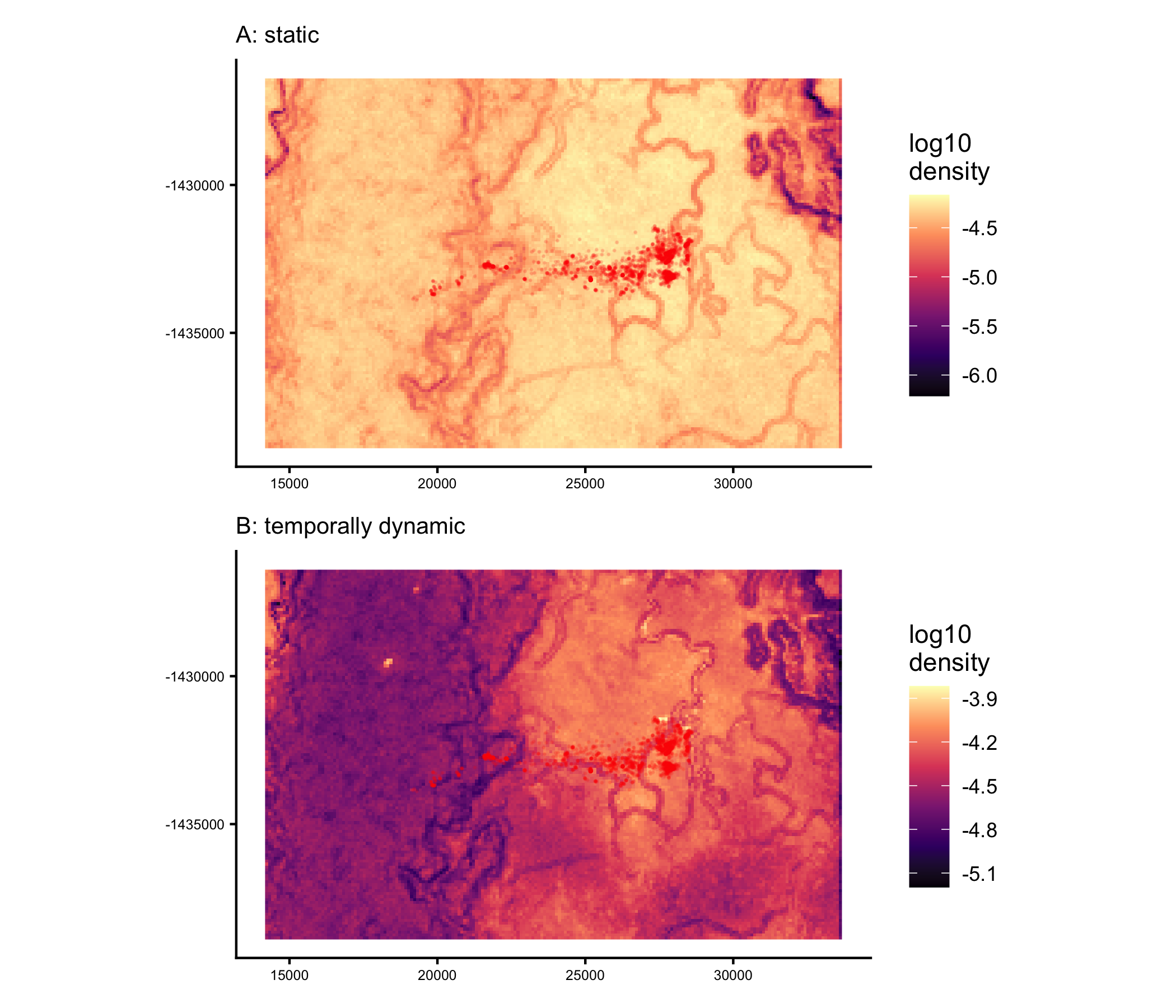
A single simulated trajectory is one realisation of a stochastic process and tells us little. The prediction is in the *ensemble*: count how often simulated animals occupy each cell of the landscape, and the result is a predicted utilisation distribution (UD).
```{r}
#| label: aggregate_function
#' Aggregate simulated locations into a normalised utilisation distribution
#'
#' @param sims       data frame of simulated locations
#' @param resolution cell size in metres
#' @param hours      optionally restrict to particular hours of the day
aggregate_to_ud <- function(sims, resolution, hours = NULL) {

  if (!is.null(hours)) sims <- sims %>% filter(hour %in% hours)

  template <- rast(extent = ext(ndvi_crop), resolution = resolution,
                   crs = crs(ndvi_crop))

  # Count the simulated locations falling in each cell
  counts <- terra::rasterize(cbind(sims$x, sims$y), template, fun = "sum")

  # Cells with no simulated locations are true zeroes, not missing data
  counts[is.na(counts)] <- 0

  # Normalise so that the layer sums to 1, making models comparable
  counts / global(counts, "sum", na.rm = TRUE)[[1]]
}
```
```{r}
#| label: build_uds
tic("Aggregating simulations")
ud_static      <- aggregate_to_ud(sims_static,      ud_res)
ud_dynamic     <- aggregate_to_ud(sims_dynamic,     ud_res)
toc()
# Check that each normalises to 1
cat("Sum of UD values - static:",
    round(global(ud_static, "sum", na.rm = TRUE)[[1]], 6),
    " dynamic:",
    round(global(ud_dynamic, "sum", na.rm = TRUE)[[1]], 6), "\n")
```
```{r}
#| label: plot_uds
#| fig-height: 6
#| fig-cap: "Predicted utilisation distributions (log scale) with observed locations in red."
plot_ud <- function(ud, title) {
  df <- as.data.frame(ud, xy = TRUE)
  names(df)[3] <- "density"

  ggplot() +
    geom_raster(data = df, aes(x = x, y = y, fill = log10(density + 1e-8))) +
    geom_point(data = buffalo_id, aes(x = x_, y = y_),
               colour = "red", size = 0.15, alpha = 0.15) +
    scale_fill_viridis_c("log10\ndensity", option = "magma") +
    coord_equal() +
    labs(title = title, x = NULL, y = NULL) +
    theme_classic() +
    theme(axis.text = element_text(size = 6),
          plot.title = element_text(size = 10))
}

plot_ud(ud_static, "A: static") / plot_ud(ud_dynamic, "B: temporally dynamic")
```
## Has the simulation converged?
How many trajectories are enough? We can answer empirically, and cheaply, by reusing the trajectories we already have: build UDs from increasing subsets and see how quickly they stabilise towards the full result.
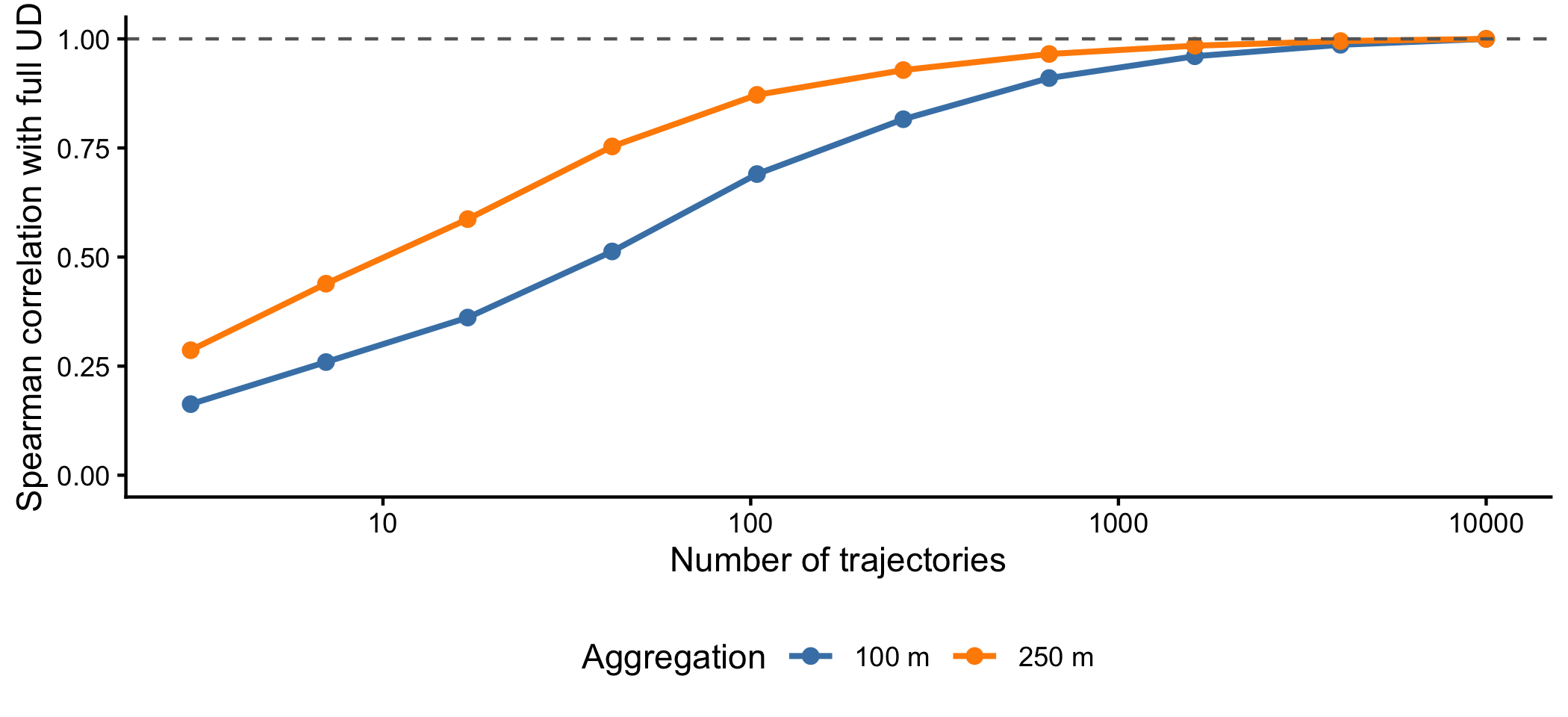
We are comparing all of the subsets to the full set - so it should start to plateau towards 1.0 as the number of trajectories increases (and ideally reach it with a subset). If it does not, the simulation has still not converged and needs more simulations.
```{r}
#| label: convergence
#| fig-height: 3.2
#| fig-cap: "Correlation between a UD built from n trajectories and the UD built from all of them."
# Subset sizes to check, kept valid for whatever `n_traj` is set to: drop any
# that exceed the number of trajectories actually simulated (they would silently
# duplicate the full set), and always include `n_traj` itself.
# subset_sizes <- c(10, 25, 50, 100, 250, 1000, 5000, n_traj)
subset_sizes <- seq(1, log(n_traj), length.out = 10) %>% exp() %>% round()
subset_sizes <- sort(unique(subset_sizes[subset_sizes <= n_traj]))

# Run the check at two aggregation resolutions, because the number of
# trajectories needed depends on how finely we are asking the question
convergence <- map_dfr(c(ud_res, ud_res_hourly), function(resolution) {
  ud_full <- aggregate_to_ud(sims_dynamic, resolution)
  map_dfr(subset_sizes, function(n) {
    ud_n <- aggregate_to_ud(sims_dynamic %>% filter(traj_id <= n), resolution)
    data.frame(
      resolution = paste0(resolution, " m"),
      n_trajectories = n,
      correlation = cor(values(ud_n)[, 1], values(ud_full)[, 1],
                        use = "complete.obs", method = "spearman")
    )
  })
})

ggplot(convergence, aes(x = n_trajectories, y = correlation, colour = resolution)) +
  geom_line(linewidth = 0.9) +
  geom_point(size = 2) +
  geom_hline(yintercept = 1, linetype = "dashed", colour = "grey40") +
  scale_x_log10("Number of trajectories") +
  scale_y_continuous("Spearman correlation with full UD", limits = c(0, 1)) +
  scale_colour_manual(values = c("steelblue", "darkorange"), name = "Aggregation") +
  theme_classic() +
  theme(legend.position = "bottom")
convergence %>% pivot_wider(names_from = resolution, values_from = correlation)
```
```{r}
#| label: convergence_verdict
# A rough rule of thumb: if a utilisation distribution built from *half* the
# trajectories already agrees closely with the full one, adding more is not
# changing the answer much. If it does not, the simulation is still moving.
half_way <- convergence %>%
  filter(n_trajectories <= n_traj / 2) %>%
  group_by(resolution) %>%
  slice_max(n_trajectories, n = 1) %>%
  ungroup() %>%
  select(resolution, n_trajectories, correlation)

half_way
```
```{r}
#| label: convergence_flag
#| echo: false
conv_fine <- half_way %>% filter(resolution == paste0(ud_res, " m")) %>% pull(correlation)
conv_coarse <- half_way %>% filter(resolution == paste0(ud_res_hourly, " m")) %>% pull(correlation)
converged <- length(conv_fine) > 0 && conv_fine > 0.95
```
::: callout-important
## Has this simulation converged?
At the `r ud_res` m aggregation, a distribution built from half the trajectories correlates `r sprintf("%.2f", conv_fine)` with the full one; at `r ud_res_hourly` m it is `r sprintf("%.2f", conv_coarse)`. `r if (converged) "That is close enough to 1 that adding more trajectories is no longer changing the answer much at this resolution." else paste0("That is well short of 1, which means **", format(n_traj, big.mark = ","), " trajectories is not yet enough** to characterise the utilisation distribution at that resolution.")`
With `r format(nrow(sims_dynamic), big.mark = ",")` simulated locations spread over a `r ud_res` m grid, each cell holds only a limited number of points, so a fine-resolution map carries more sampling noise than a coarse one — which is exactly what the gap between the two curves shows.
Two levers are available if the answer is still moving, and the second curve shows the second of them:
- **More trajectories.** @Forrest2025-le used 100,000 trajectories of 3,000 steps, run on a computing cluster. Increase `n_traj` in the parameter block.
- **Coarser aggregation.** The same simulations converge faster at `r ud_res_hourly` m, because each cell collects more points. If the ecological question does not require `r ud_res` m resolution, this is free.
Run this check before interpreting anything downstream. Nothing about the utilisation distribution maps themselves reveals whether they have settled — they can look equally plausible either way.
Note also that this is a *self-consistency* check: it asks whether the answer has stopped changing, not whether it is right. A converged UD can still be a converged estimate of a bad model.
:::
## Hourly utilisation distributions
The dynamic model's real claim is not just about where the animal goes, but about *when*. We therefore also aggregate separately for each hour of the day.
```{r}
#| label: hourly_uds
tic("Building hourly UDs")
uds_hourly_static  <- rast(map(0:23, ~ aggregate_to_ud(sims_static,  ud_res_hourly, hours = .x)))
uds_hourly_dynamic <- rast(map(0:23, ~ aggregate_to_ud(sims_dynamic, ud_res_hourly, hours = .x)))
toc()
names(uds_hourly_static)  <- paste0("hour_", 0:23)
names(uds_hourly_dynamic) <- paste0("hour_", 0:23)

uds_hourly_dynamic
```
```{r}
#| label: hourly_ud_gif
#| results: hide
ud_gif_path <- file.path(figure_save_path, "hourly_uds.gif")

# A shared colour scale across all frames, on the log scale
hourly_vals <- values(uds_hourly_dynamic)
ud_limits <- range(log10(hourly_vals[hourly_vals > 0]), na.rm = TRUE)

ud_frames <- map_chr(0:23, function(h) {
  f <- file.path(plot_save_path, sprintf("ud_frame_%02d.png", h))
  png(f, width = 150, height = 150, units = "mm", res = 150)
  plot(log10(uds_hourly_dynamic[[h + 1]]),
       main = sprintf("Predicted use, %02d:00", h),
       range = ud_limits, col = viridis(100, option = "magma"))
  dev.off()
  f
})

image_read(ud_frames) %>%
  image_animate(fps = 4) %>%
  image_write(ud_gif_path)

unlink(ud_frames)
```
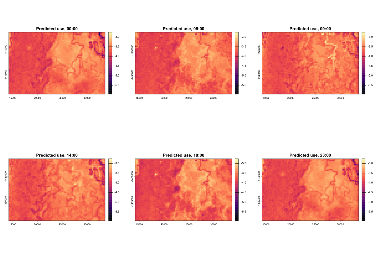
Predicted use for the dynamic model is not a fixed map but a landscape that shifts through the day, as the simulated animals move between the habitats they select at different times.
# 10. Hourly summaries — does the simulated behaviour match?
Before asking whether the models predict the right *places*, it is worth asking whether they reproduce the right *behaviour*. We extract covariate values at the simulated locations and compare hourly summaries against the observed data.
```{r}
#| label: extract_sim_covariates
tic("Extracting covariates at simulated locations")
sims_combined <- bind_rows(sims_static, sims_dynamic)

sim_covs <- sims_combined %>%
  mutate(covariate_values = terra::extract(covariates, cbind(x, y))) %>%
  unpack(covariate_values) %>%
  filter(!is.na(ndvi), !is.na(canopy), !is.na(slope))
toc()
head(sim_covs)
```
With a single individual there is no between-animal variation to display, so a single observed curve would appear to have no uncertainty at all. To give a fair sense of the observed variability, we split the observed track into weekly blocks and compute hourly means within each — giving a distribution of observed curves comparable to the distribution of simulated ones.
```{r}
#| label: hourly_summaries
# Observed: hourly means within each week.
# We work from the *steps* rather than the raw locations, and take covariates at
# the end point of each step - exactly how the model treats a used step, and
# directly comparable to the simulated locations, which are also step endpoints.
observed_steps_covs <- buffalo_steps %>%
  mutate(covariate_values = terra::extract(covariates, cbind(x2_, y2_))) %>%
  unpack(covariate_values) %>%
  mutate(hour = hour(t1_),
         week = as.integer(difftime(t1_, min(t1_), units = "days")) %/% 7) %>%
  filter(!is.na(ndvi), !is.na(canopy), !is.na(slope))

observed_hourly <- observed_steps_covs %>%
  group_by(week, hour) %>%
  summarise(ndvi   = mean(ndvi),
            canopy = mean(canopy),
            slope  = mean(slope),
            sl     = mean(sl_),
            .groups = "drop") %>%
  mutate(model = "Observed", unit = paste0("week_", week))

# Simulated: hourly means within each trajectory
simulated_hourly <- sim_covs %>%
  group_by(model, traj_id, hour) %>%
  summarise(ndvi = mean(ndvi, na.rm = TRUE),
            canopy = mean(canopy, na.rm = TRUE),
            slope = mean(slope, na.rm = TRUE),
            sl = mean(sl, na.rm = TRUE),
            .groups = "drop") %>%
  mutate(unit = paste0(model, "_", traj_id))

hourly_long <- bind_rows(
  observed_hourly %>% select(model, unit, hour, ndvi, canopy, slope, sl),
  simulated_hourly %>% select(model, unit, hour, ndvi, canopy, slope, sl)
) %>%
  pivot_longer(c(ndvi, canopy, slope, sl),
               names_to = "variable", values_to = "value")

# Quantiles across units, for each model, hour and variable
hourly_quantiles <- hourly_long %>%
  group_by(model, variable, hour) %>%
  summarise(mean = mean(value, na.rm = TRUE),
            q025 = quantile(value, 0.025, na.rm = TRUE),
            q25  = quantile(value, 0.25,  na.rm = TRUE),
            q75  = quantile(value, 0.75,  na.rm = TRUE),
            q975 = quantile(value, 0.975, na.rm = TRUE),
            .groups = "drop")
```
```{r}
#| label: plot_hourly_summaries
#| fig-height: 5.5
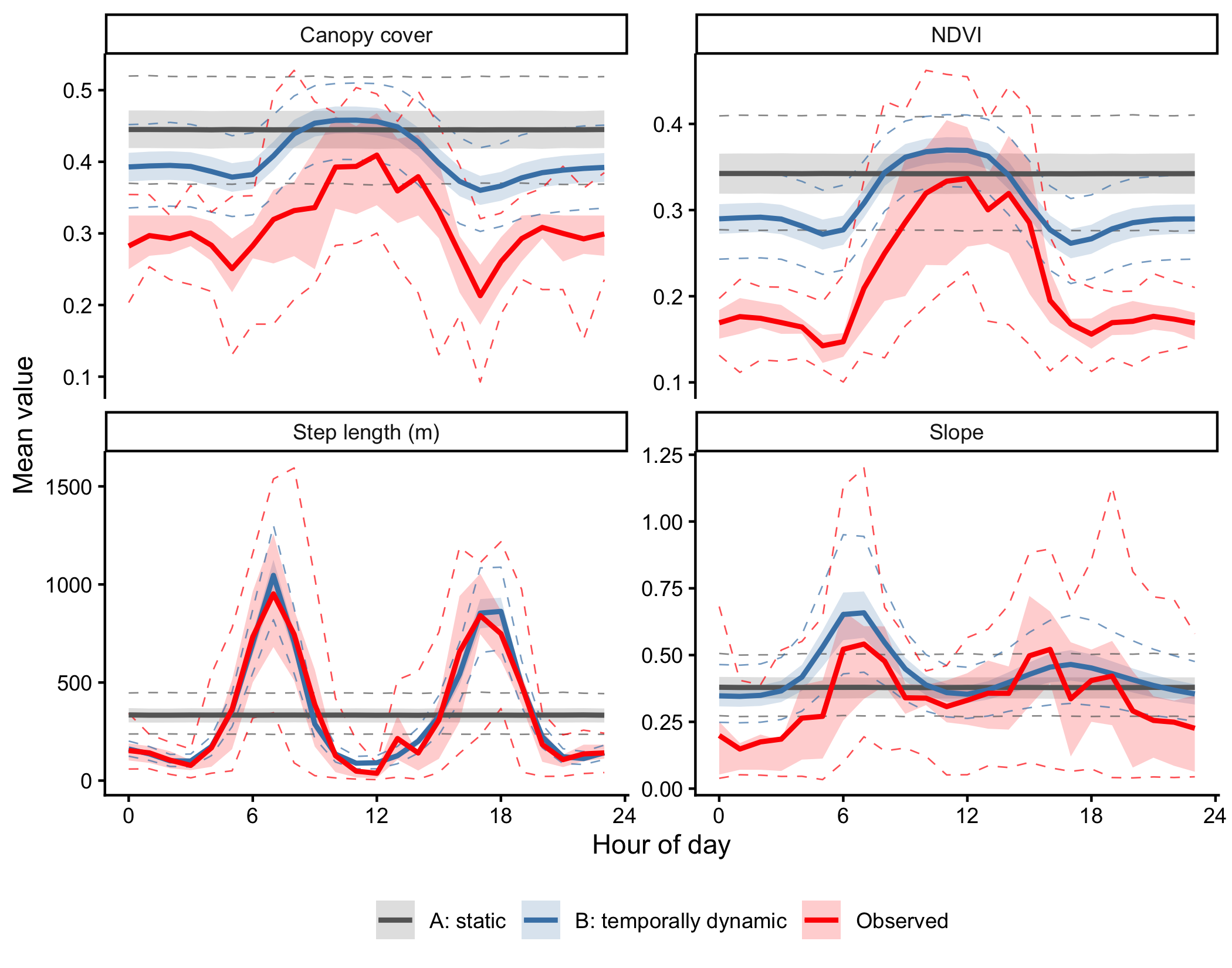
#| fig-cap: "Hourly mean step length and habitat use. Ribbons show the 50% interval across simulated trajectories (or observed weeks); dashed lines the 95% interval; solid lines the mean."
model_colours <- c("A: static" = "grey40",
                   "B: temporally dynamic" = "steelblue",
                   "Observed" = "red")

variable_labels <- c(sl = "Step length (m)", ndvi = "NDVI",
                     canopy = "Canopy cover", slope = "Slope")

ggplot() +
  geom_ribbon(data = hourly_quantiles,
              aes(x = hour, ymin = q25, ymax = q75, fill = model),
              alpha = 0.2) +
  geom_line(data = hourly_quantiles,
            aes(x = hour, y = q025, colour = model),
            linetype = "dashed", linewidth = 0.3, alpha = 0.7) +
  geom_line(data = hourly_quantiles,
            aes(x = hour, y = q975, colour = model),
            linetype = "dashed", linewidth = 0.3, alpha = 0.7) +
  geom_line(data = hourly_quantiles,
            aes(x = hour, y = mean, colour = model),
            linewidth = 1) +
  facet_wrap(~ variable, scales = "free_y",
             labeller = labeller(variable = variable_labels)) +
  scale_colour_manual(values = model_colours, name = NULL) +
  scale_fill_manual(values = model_colours, name = NULL) +
  scale_x_continuous("Hour of day", breaks = seq(0, 24, 6)) +
  labs(y = "Mean value") +
  theme_classic() +
  theme(legend.position = "bottom")
```
The static model produces flat lines for everything, which is the only thing it can do. The dynamic model tracks the shape of the observed daily cycles. The match is not perfect — the simulated animals roam over the whole landscape while the observed animal was confined to part of it, so the absolute levels differ — but the *timing* of activity and habitat use is recovered.
# 11. Assessing the predictions
Finally, the question the whole pipeline was built to answer: do the predicted utilisation distributions match where the animal actually was?
**Note that we are using the same data to build the model and to validate it.** This is not a proper out-of-sample validation, and the results are therefore optimistic. A proper validation would require a second animal, or a second year of data from the same animal. Here we just illustrate the process.
## The Boyce index
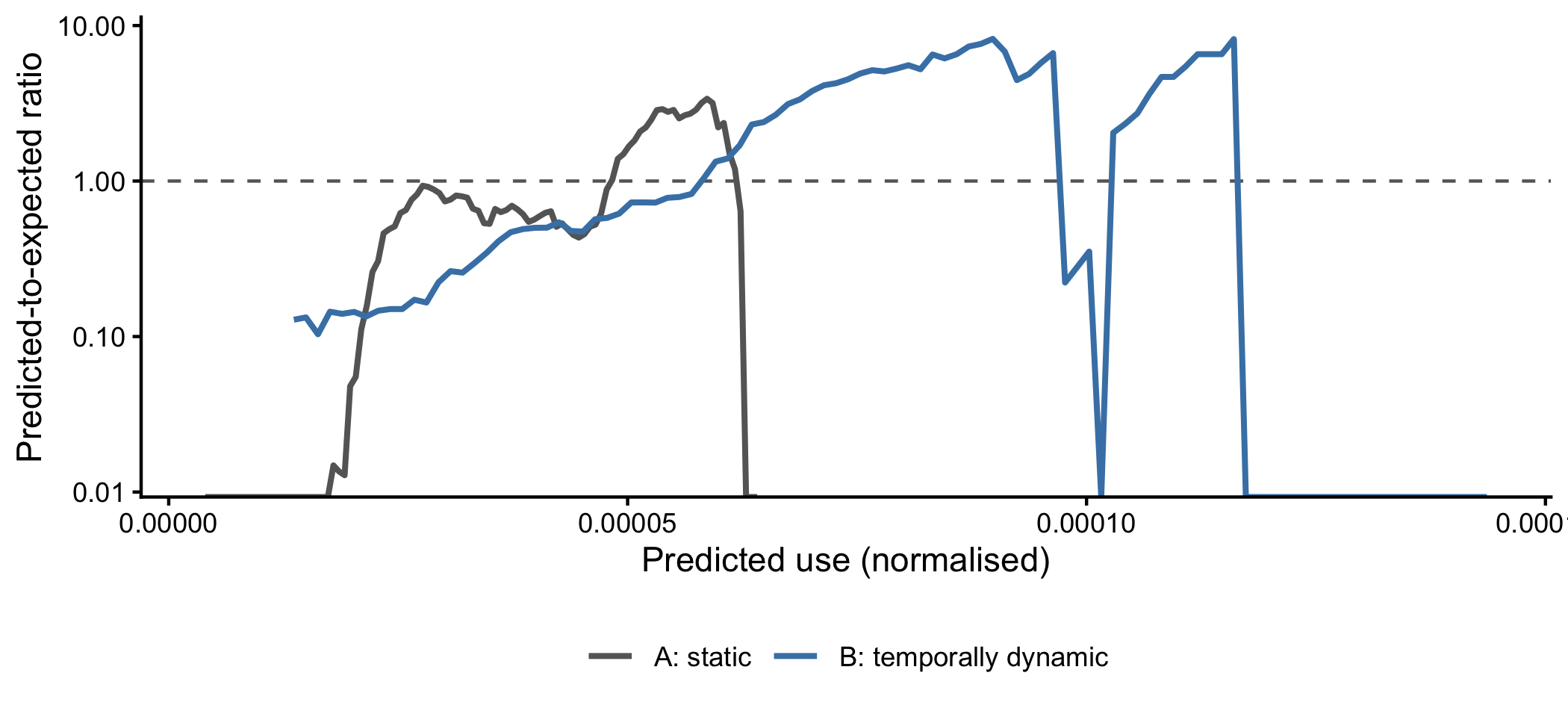
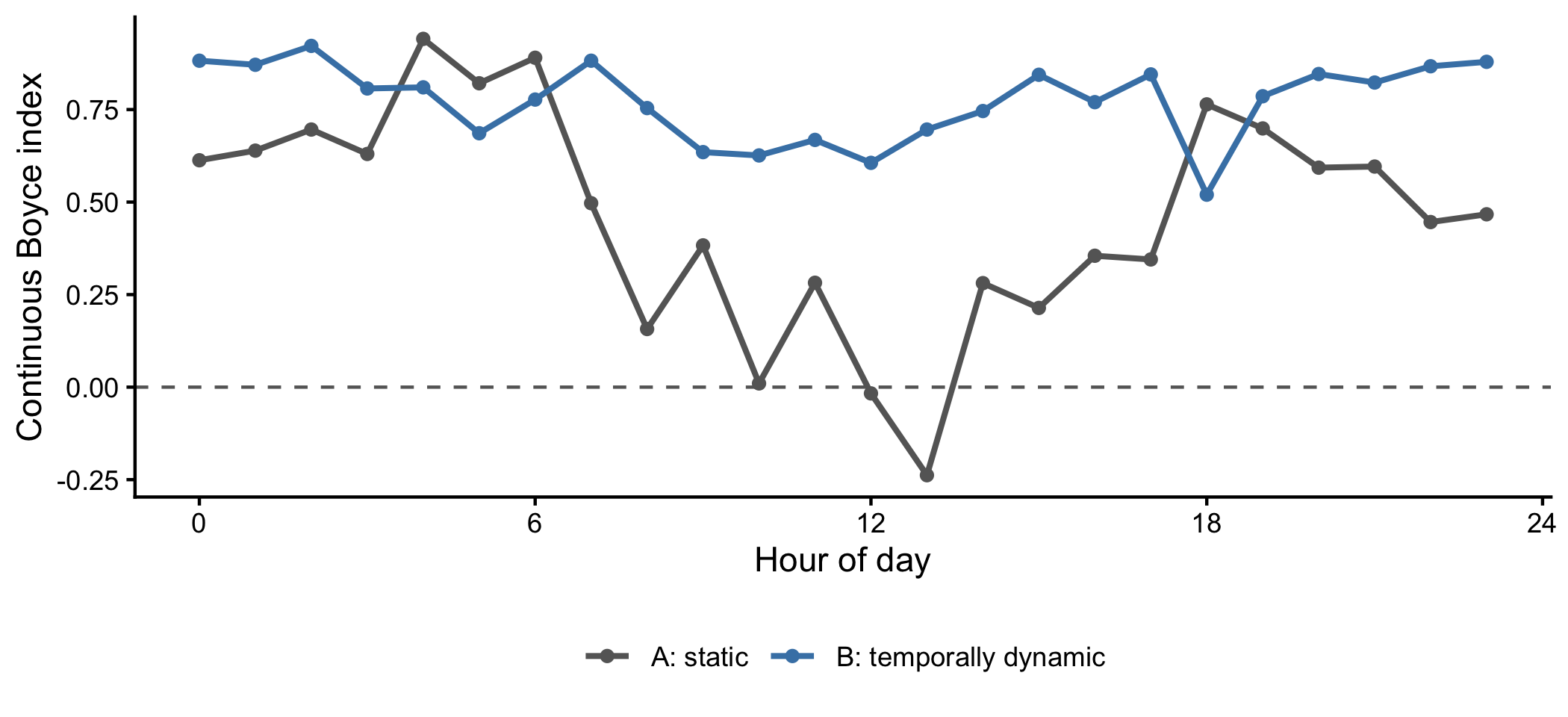
For presence-only data a standard tool is the **continuous Boyce index** [@Boyce2002-xr; @Hirzel2006-hu]. It divides the range of predicted values into overlapping bins and, for each, computes the ratio of observed locations to the area available at that predicted value. For a good model this ratio increases monotonically with the prediction: places predicted to be used more, are used more.
The index itself is the rank (Spearman) correlation between that ratio and the predicted value. It ranges from −1 to 1, where values near zero indicate a model no better than random.
```{r}
#| label: boyce_function
#' Compute Boyce index statistics for a predicted surface
#'
#' @param ud  predicted utilisation distribution
#' @param obs two-column matrix of observed locations
compute_boyce <- function(ud, obs) {

  # Predicted values at the observed locations
  obs_vals <- terra::extract(ud, obs)[, 1]
  obs_vals <- obs_vals[!is.na(obs_vals)]

  # Predicted values across the whole landscape (the "available" set)
  all_vals <- terra::values(ud, na.rm = TRUE)[, 1]
  all_vals <- all_vals[!is.na(all_vals)]

  # With few observed locations - which can happen for a single hour of the day -
  # the index is not meaningful, so return NA rather than a misleading number
  if (length(obs_vals) < 10 || length(unique(all_vals)) < 10) {
    return(list(spearman = NA_real_, pearson = NA_real_,
                F_ratio = data.frame(HS = numeric(0), F.ratio = numeric(0))))
  }

  window_width <- (max(all_vals) - min(all_vals)) / 10

  safe_boyce <- function(method) {
    out <- try(ecospat::ecospat.boyce(all_vals, obs_vals,
                                      window.w = window_width, res = 100,
                                      method = method, PEplot = FALSE),
               silent = TRUE)
    if (inherits(out, "try-error")) NULL else out
  }

  bi_spearman <- safe_boyce("spearman")
  bi_pearson  <- safe_boyce("pearson")

  list(
    spearman = if (is.null(bi_spearman)) NA_real_ else bi_spearman$cor,
    pearson  = if (is.null(bi_pearson))  NA_real_ else bi_pearson$cor,
    F_ratio  = if (is.null(bi_spearman)) data.frame(HS = numeric(0), F.ratio = numeric(0))
               else data.frame(HS = bi_spearman$HS, F.ratio = bi_spearman$F.ratio)
  )
}
```
```{r}
#| label: boyce_overall
obs_locations <- cbind(buffalo_id$x_, buffalo_id$y_)

boyce_static  <- compute_boyce(ud_static,  obs_locations)
boyce_dynamic <- compute_boyce(ud_dynamic, obs_locations)

boyce_results <- tibble(
  model    = c("A: static", "B: temporally dynamic"),
  spearman = c(boyce_static$spearman, boyce_dynamic$spearman),
  pearson  = c(boyce_static$pearson,  boyce_dynamic$pearson)
)

boyce_results
```
## Is that number stable?
Before reading anything into those figures, we should ask whether they would come out the same again. The convergence check told us the utilisation distributions are still noisy, and a Boyce index computed on a noisy surface is itself noisy.
A cheap way to find out, using only the simulations we already have: split the trajectories into two halves, build a utilisation distribution from each, and compute the index separately for both. Two halves of the same simulation, under the same model, should agree.
```{r}
#| label: boyce_stability
split_half_boyce <- map_dfr(
  list("A: static" = sims_static, "B: temporally dynamic" = sims_dynamic),
  function(sims) {
    half_1 <- sims %>% filter(traj_id <= n_traj / 2)
    half_2 <- sims %>% filter(traj_id >  n_traj / 2)
    data.frame(
      half_1 = compute_boyce(aggregate_to_ud(half_1, ud_res), obs_locations)$spearman,
      half_2 = compute_boyce(aggregate_to_ud(half_2, ud_res), obs_locations)$spearman
    )
  }, .id = "model") %>%
  mutate(difference = abs(half_1 - half_2))

split_half_boyce
```
```{r}
#| label: plot_f_ratio
#| fig-height: 3.2
#| fig-cap: "Predicted-to-expected ratio against predicted habitat suitability. A well-calibrated model rises monotonically above the dashed line at 1."
bind_rows(
  boyce_static$F_ratio  %>% mutate(model = "A: static"),
  boyce_dynamic$F_ratio %>% mutate(model = "B: temporally dynamic")
) %>%
  ggplot(aes(x = HS, y = F.ratio, colour = model)) +
  geom_hline(yintercept = 1, linetype = "dashed", colour = "grey40") +
  geom_line(linewidth = 0.9) +
  scale_colour_manual(values = model_colours, name = NULL) +
  scale_x_continuous("Predicted use (normalised)") +
  scale_y_log10("Predicted-to-expected ratio") +
  theme_classic() +
  theme(legend.position = "bottom")
```
The F-ratio curve is more informative than the single index value, because it shows *where* a model succeeds or fails. A model can achieve a respectable correlation while badly over-predicting use in the very highest-suitability cells, and that shows up here as a curve that flattens or turns down at the right-hand end.
## Validation by hour of day
The overall UD averages over the day, but we can also check hour by hour. For each hour, we compare that hour's predicted UD against the locations the animal actually occupied at that hour.
**Note that in this case, our simulated trajectories are split into 24 (hourly) groups, meaning each of the hourly UDs are created with 1/24 of the number of locations, which may be a lot noisier depending on the number of trajectories simulated.**
```{r}
#| label: hourly_validation
observed_by_hour <- buffalo_id %>% mutate(hour = hour(t_))

hourly_validation <- map_dfr(0:23, function(h) {

  obs_h <- observed_by_hour %>% filter(hour == h)
  obs_h_mat <- cbind(obs_h$x_, obs_h$y_)

  bi_static  <- compute_boyce(uds_hourly_static[[h + 1]],  obs_h_mat)
  bi_dynamic <- compute_boyce(uds_hourly_dynamic[[h + 1]], obs_h_mat)

  data.frame(
    hour = h,
    n_observed = nrow(obs_h),
    `A: static` = bi_static$spearman,               # change to pearson if desired
    `B: temporally dynamic` = bi_dynamic$spearman,  # change to pearson if desired
    check.names = FALSE
  )
})

hourly_validation
```
Instead of plotting the F-ratio curves for every hour, we just show the Spearman rank correlation for each hour (this can be switched out for the Pearson correlation in the chunk above).
```{r}
#| label: plot_hourly_validation
#| fig-height: 3.2
#| fig-cap: "Continuous Boyce index by hour of day for each model."
hourly_validation %>%
  pivot_longer(c(`A: static`, `B: temporally dynamic`),
               names_to = "model", values_to = "boyce") %>%
  ggplot(aes(x = hour, y = boyce, colour = model)) +
  geom_hline(yintercept = 0, linetype = "dashed", colour = "grey40") +
  geom_line(linewidth = 0.9) +
  geom_point(size = 1.5) +
  scale_colour_manual(values = model_colours, name = NULL) +
  scale_x_continuous("Hour of day", breaks = seq(0, 24, 6)) +
  scale_y_continuous("Continuous Boyce index") +
  theme_classic() +
  theme(legend.position = "bottom")
```
```{r}
#| label: hourly_validation_summary
hourly_validation %>%
  summarise(
    mean_static  = mean(`A: static`, na.rm = TRUE),
    mean_dynamic = mean(`B: temporally dynamic`, na.rm = TRUE),
    hours_dynamic_better = sum(`B: temporally dynamic` > `A: static`, na.rm = TRUE),
    hours_compared = sum(!is.na(`A: static`) & !is.na(`B: temporally dynamic`))
  )
```
# 12. Doing the same thing with `amt`
Everything above simulates by hand, so that each part of the redistribution kernel is visible. In practice, `amt` implements this directly [@Signer2023-wm], and for a static model you can go from a fitted object to simulated paths in a few lines.
```{r}
#| label: amt_simulation
# The movement distributions amt derives from the fitted model - these should
# match the values we computed by hand in section 6
amt_sl_distr <- amt::update_sl_distr(ssf_static)
amt_ta_distr <- amt::update_ta_distr(ssf_static)

cat("amt    - shape:", round(amt_sl_distr$params$shape, 6),
    " scale:", round(amt_sl_distr$params$scale, 4),
    " kappa:", round(amt_ta_distr$params$kappa, 6), "\n")
cat("manual - shape:", round(hourly_coefs_static$shape[1], 6),
    " scale:", round(hourly_coefs_static$scale[1], 4),
    " kappa:", round(hourly_coefs_static$kappa[1], 6), "\n")
```
## Building a redistribution kernel
Two details are needed to make this work, and both are worth knowing about because neither is obvious from the error messages you get without them.
**The extraction function.** By default `redistribution_kernel()` extracts covariates at *both* ends of each step, producing columns named `ndvi_start` and `ndvi_end`. Our model refers simply to `ndvi`, so we supply a custom `fun` that extracts at the end of the step only. That function also has to compute the derived movement terms `log_sl_` and `cos_ta_`, since the kernel provides only `sl_` and `ta_`.
**The extent.** We use the *full* covariate rasters here rather than the cropped simulation extent. `amt` terminates a path once too many proposed steps fall outside the map — on our subset crop, paths soon terminate.
```{r}
#| label: amt_redistribution_kernel
start_step <- ssf_data %>% filter(case_) %>% slice(1)

rk <- amt::redistribution_kernel(
  ssf_static,
  map       = covariates,                     # full extent, so paths do not hit the edge
  start     = amt::make_start(start_step),
  n.control = 500,
  landscape = "continuous",
  tolerance.outside = 0.2,
  fun = function(xy, map) {
    amt::extract_covariates(xy, map, where = "end") %>%
      mutate(log_sl_ = log(sl_), cos_ta_ = cos(ta_))
  })

tic("amt simulation")
amt_paths <- map_dfr(1:10, function(i) {
  amt::simulate_path(rk, n.steps = 500) %>%
    as.data.frame() %>%
    mutate(traj_id = i)
})
toc()
cat("Rows:", nrow(amt_paths),
    " | steps completed per trajectory:",
    paste(unique(table(amt_paths$traj_id)), collapse = ", "), "\n")
head(amt_paths)
```
```{r}
#| label: amt_comparison
#| fig-height: 4.5
#| fig-cap: "Paths simulated with `amt::simulate_path()` from the static model, over the full landscape. The dashed box is the extent used for our own simulations."
# The full NDVI layer, coarsened for plotting
ndvi_full_df <- as.data.frame(terra::aggregate(ndvi, fact = 8, fun = "mean"), xy = TRUE)

ggplot() +
  geom_raster(data = ndvi_full_df, aes(x = x, y = y, fill = ndvi)) +
  annotate("rect",
           xmin = xmin(ndvi_crop), xmax = xmax(ndvi_crop),
           ymin = ymin(ndvi_crop), ymax = ymax(ndvi_crop),
           fill = NA, colour = "white", linetype = "dashed", linewidth = 0.4) +
  geom_path(data = amt_paths,
            aes(x = x_, y = y_, colour = factor(traj_id)),
            alpha = 0.8, linewidth = 0.25) +
  scale_fill_gradientn(colours = brewer.pal(9, "Greens"), name = "NDVI") +
  scale_colour_viridis_d(guide = "none") +
  coord_equal() +
  labs(x = "Easting (m)", y = "Northing (m)") +
  theme_classic()
```
## Why we wrote the sampler by hand
`amt::redistribution_kernel()` builds its kernel from **one** fitted model evaluated against a **fixed** map. That is exactly right for a static model, and it is the tool to reach for in that case. Our dynamic model, though, has coefficients that change every hour — so there is no single set of coefficients, and no single habitat surface, to hand it.
The custom `fun` above is most of the way to a solution. Since it receives the proposed steps, including their timestamps, it can select the layer matching the hour rather than using a fixed map:
```{r}
#| label: amt_custom_fun
#| eval: false
# Sketch: an extraction function that indexes the 24-layer stack of hourly
# selection surfaces by the hour of the proposed step. Because the surfaces
# already contain the linear predictor, the model passed to the kernel would be
# one whose single habitat covariate is `selection`, with a coefficient of 1.
hourly_extract <- function(xy, map) {
  h <- lubridate::hour(xy$t_)
  xy %>%
    mutate(
      selection = map_dbl(seq_len(nrow(xy)), function(i) {
        terra::extract(map[[h[i] + 1]], cbind(xy$x_[i], xy$y_[i]))[, 1]
      }),
      log_sl_ = log(sl_),
      cos_ta_ = cos(ta_)
    )
}
```
That works, but note what it costs: a per-row `terra::extract()` call, which is the overhead our matrix lookup in section 8 was written to avoid. The alternative is to rebuild the kernel for each hour and step through them.
# Summary
Starting from a single animal's GPS trajectory and three environmental layers, we:
1. Generated used and available steps, and fitted **two** step selection functions — a static one and a temporally dynamic GAM with cyclic smooths.
2. Reduced both models to a common representation: a table of habitat coefficients and corrected movement parameters for each hour of the day, cross-checked against `amt`.
3. Pre-computed hourly habitat selection surfaces and simulated stochastic trajectories from each model, being explicit about how the choice of starting location and boundary determines what question the simulation answers.
4. Aggregated those trajectories into utilisation distributions, overall and by hour, and checked that the number of trajectories was sufficient.
5. Compared simulated and observed hourly movement and habitat use.
6. Validated the predicted distributions against the observed locations, overall and hour by hour.
The dynamic model was preferred by AIC, reproduced the observed daily activity cycle that the static model cannot represent at all, and scored substantially better hour by hour. But the whole-day comparison was more similar.
## References
::: {#refs}
:::
## Session info
```{r}
#| label: session_info
sessionInfo()
```