Exploration of temporal dynamics

Abstract

In this script we demonstrate different approaches to including covariates in an SSF model.

Load required packages

library(tidyverse)
packages <- c("amt", "sf", "terra", "RColorBrewer", "leaflet")
walk(packages, require, character.only = T)

Import data and clean

buffalo_data <- read_csv("data/buffalo.csv") 

New names:
Rows: 133161 Columns: 11
── Column specification
──────────────────────────────────────────────────────── Delimiter: "," chr
(2): node, dates dbl (7): ...1, lat, lon, height, accuracy, heading, speed dttm
(2): timestamp, DateTime
ℹ Use `spec()` to retrieve the full column specification for this data. ℹ
Specify the column types or set `show_col_types = FALSE` to quiet this message.
• `` -> `...1`

# remove individuals that have poor data quality or less than about 3 months of data. 
# The "2014.GPS_COMPACT copy.csv" string is a duplicate of ID 2024, so we exclude it
buffalo_data <- buffalo_data %>% filter(!node %in% c("2014.GPS_COMPACT copy.csv", 
                                           2029, 2043, 2265, 2284, 2346))

buffalo_data <- buffalo_data %>%  
  group_by(node) %>% 
  arrange(DateTime, .by_group = T) %>% 
  distinct(DateTime, .keep_all = T) %>% 
  arrange(node) %>% 
  mutate(ID = node)

buffalo_clean <- buffalo_data[, c(12, 2, 4, 3)]
colnames(buffalo_clean) <- c("id", "time", "lon", "lat")
attr(buffalo_clean$time, "tzone") <- "Australia/Queensland"
head(buffalo_clean)

tz(buffalo_clean$time)

[1] "Australia/Queensland"

buffalo_ids <- unique(buffalo_clean$id)

Create a step object

Use the amt package to create a trajectory object from the cleaned data.

buffalo_all <- buffalo_clean %>% mk_track(id = id,
                                           lon,
                                           lat, 
                                           time, 
                                           all_cols = T,
                                           crs = 4326) %>% 
  transform_coords(crs_to = 3112, crs_from = 4326) # Transformation to GDA94 / 
# Geoscience Australia Lambert (https://epsg.io/3112)

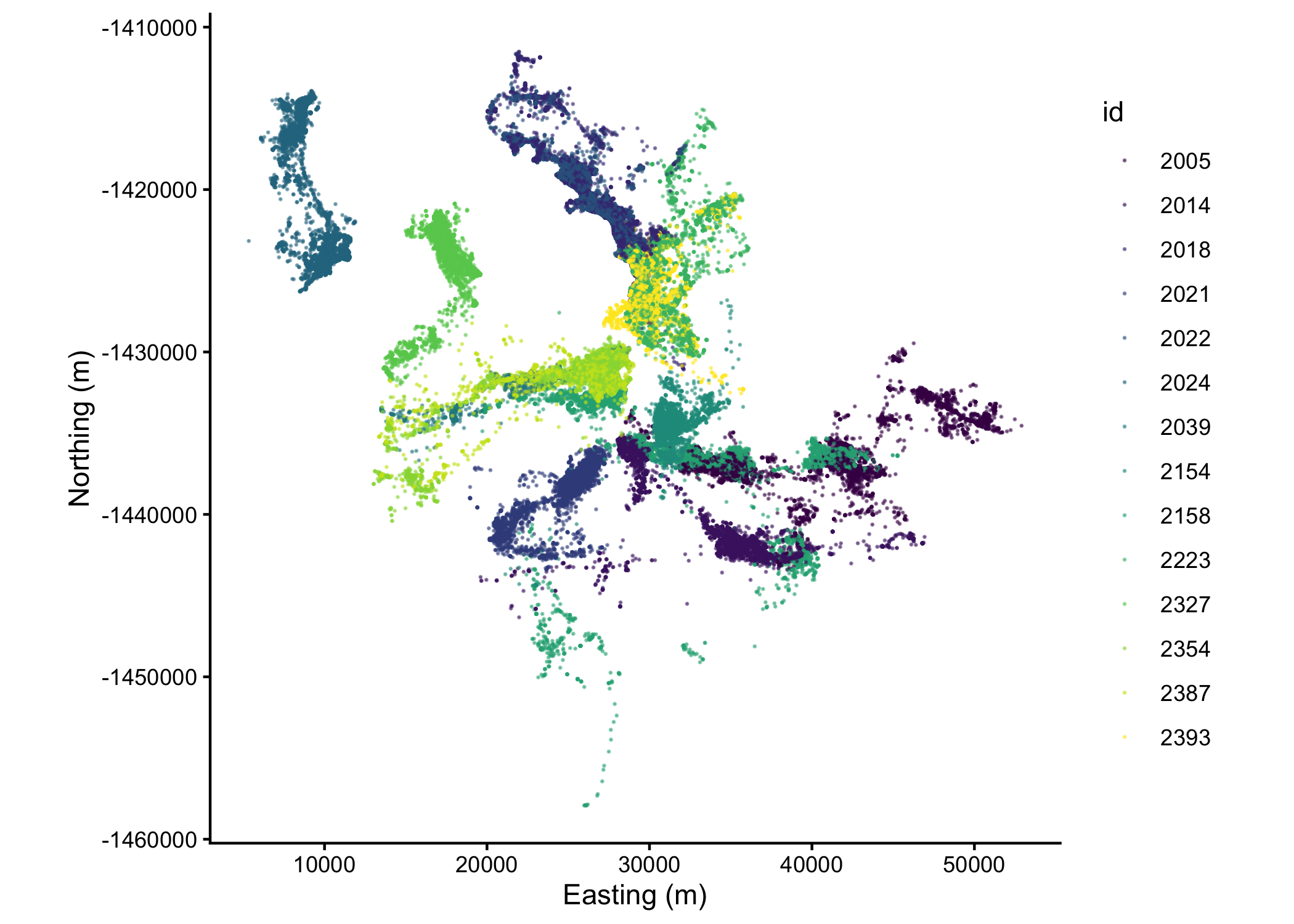
Plot the data spatially

buffalo_all %>%
  ggplot(aes(x = x_, y = y_, colour = id)) +
  geom_point(alpha = 0.5, size = 0.1) + 
  coord_fixed() +
  scale_x_continuous("Easting (m)") +
  scale_y_continuous("Northing (m)") +
  scale_colour_viridis_d() +
  theme_classic() +
  theme(legend.position = "right") 

# ggsave("outputs/data_prep/buffalo_djelk_map.png",
#        width = 150, height = 150, units = "mm",  dpi = 600)

Show data on a satellite basemap

If viewing as a PDF this will be an automated screenshot. It viewing the HTML file this should be interactive.

# Use the original longitude/latitude data for mapping
leaflet(data = buffalo_clean) %>%
  addProviderTiles(providers$Esri.WorldImagery) %>%
  addCircleMarkers(
    lng = ~lon, lat = ~lat,
    color = "red", radius = 0.5, opacity = 0.5,
    popup = ~paste("ID:", id, "<br>", "Time:", time)
  ) %>%
  addLayersControl(
    baseGroups = c("Satellite"),
    options = layersControlOptions(collapsed = TRUE)
  )

Pick out a single individual

which_buffalo <- "2158" # select a single buffalo ID

buffalo_id <- buffalo_all %>% filter(id == which_buffalo)

buffalo_id %>%
  ggplot(aes(x = x_, y = y_, colour = t_)) +
  geom_path(alpha = 0.5) + 
  geom_point(alpha = 0.5, size = 0.1) + 
  coord_fixed() +
  scale_x_continuous("Easting (m)") +
  scale_y_continuous("Northing (m)") +
  theme_classic()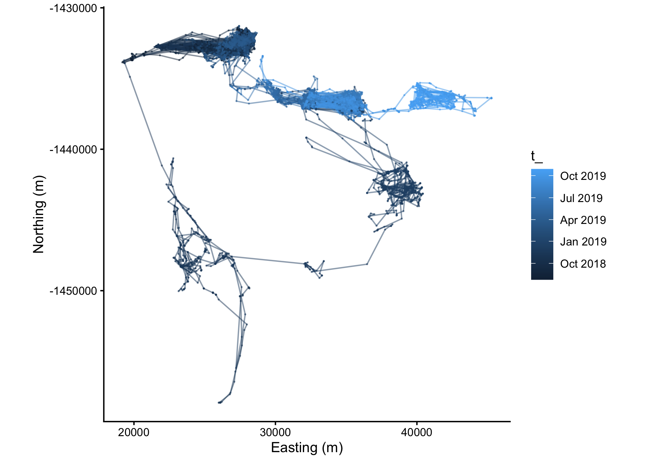

Create steps

We will just use a steps object here for now

buffalo_id_steps <- buffalo_id %>% 
  steps()

head(buffalo_id_steps)

Import spatial covariates

NDVI

Although NDVI changes over time, and we have access to monthly layers, we will just select a single month here.

ndvi <- rast("mapping/ndvi_aug_2018.tif")
plot(ndvi, main = "NDVI August 2018")
points(buffalo_id$x_, buffalo_id$y_, col = "red", pch = 16, cex = 0.5)

ndvi

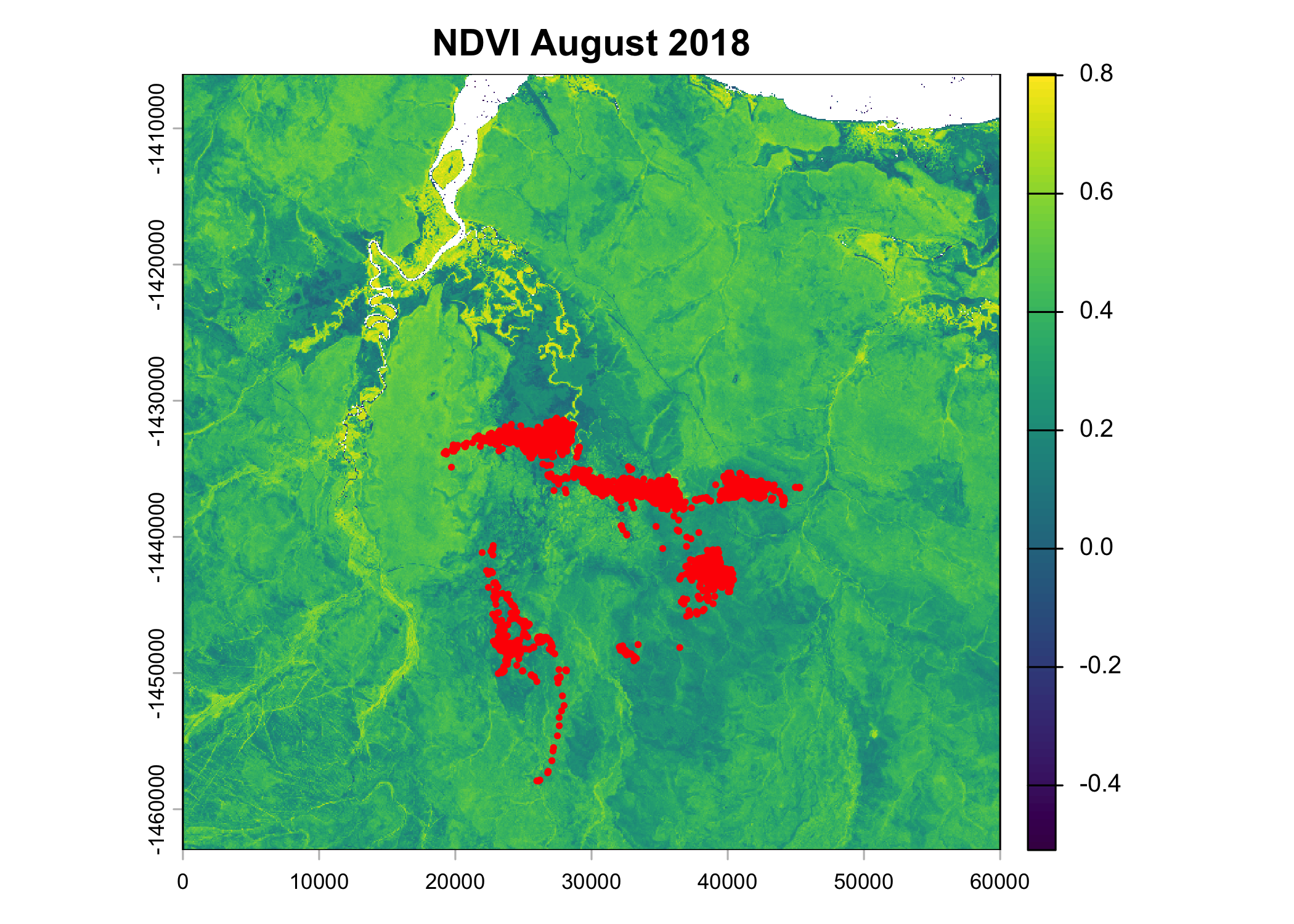
class       : SpatRaster
size        : 2280, 2400, 1  (nrow, ncol, nlyr)
resolution  : 25, 25  (x, y)
extent      : 0, 60000, -1463000, -1406000  (xmin, xmax, ymin, ymax)
coord. ref. : GDA94 / Geoscience Australia Lambert (EPSG:3112)
source      : ndvi_aug_2018.tif
name        :      ndvi
min value   : -0.544105
max value   :  0.808655

Other covariates

canopy <- rast("mapping/canopy_cover.tif")/100
herby <- rast("mapping/veg_herby.tif")
slope <- rast("mapping/slope_raster.tif")

spatial_covs <- c(ndvi, canopy, herby, slope)
names(spatial_covs) <- c("ndvi", "canopy", "herby", "slope")
plot(spatial_covs)

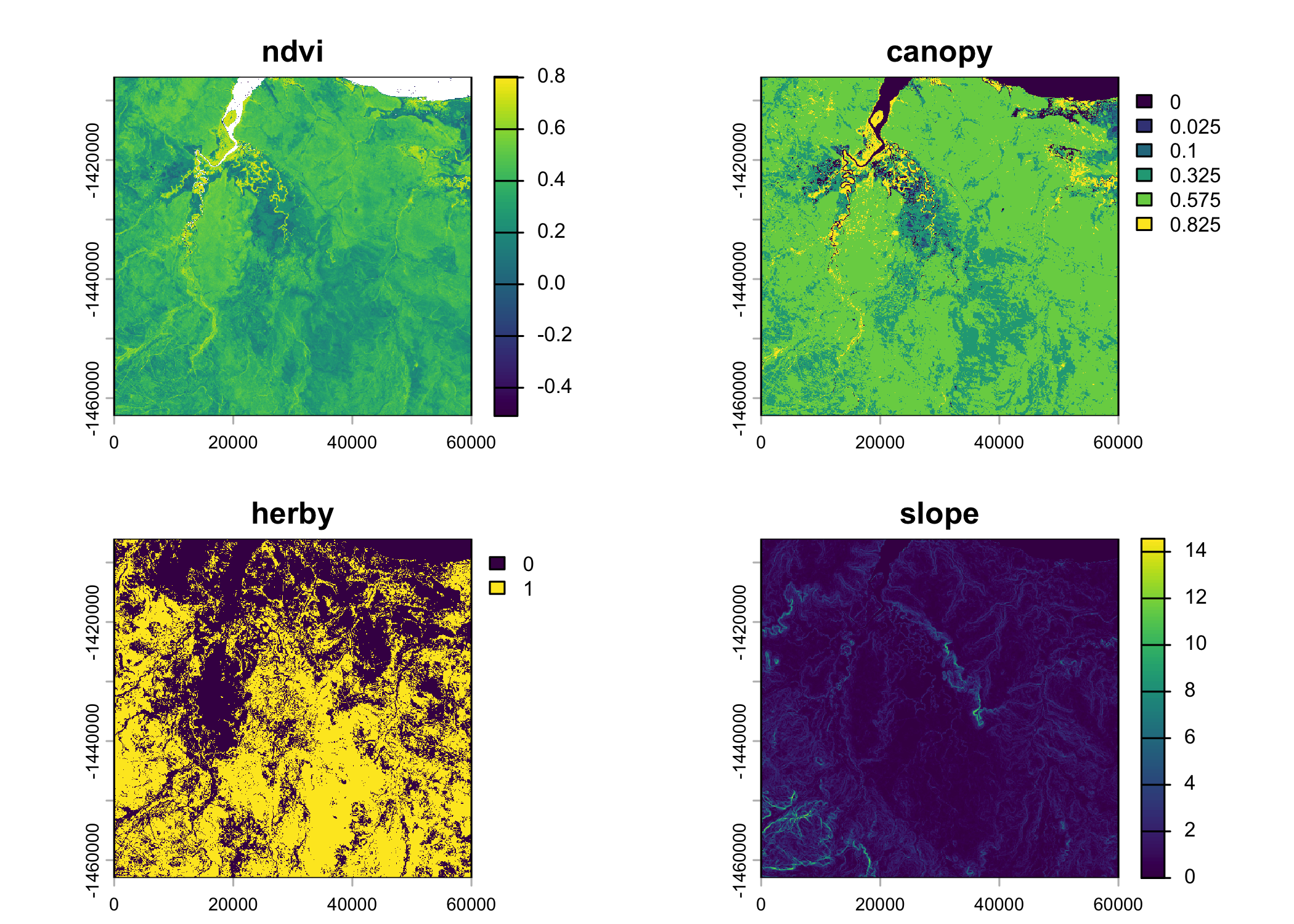
Crop covariates to the range of data to determine the background values

study_area <- st_as_sf(buffalo_id, coords = c("x_", "y_"), crs = 3112) %>% 
  st_buffer(5000) # buffer to ensure we capture the background values]

spatial_covs_cropped <- spatial_covs %>% 
  terra::crop(terra::ext(study_area))

plot(spatial_covs_cropped$ndvi, main = "Cropped NDVI")
points(buffalo_id$x_, buffalo_id$y_, col = "red", pch = 16, cex = 0.5)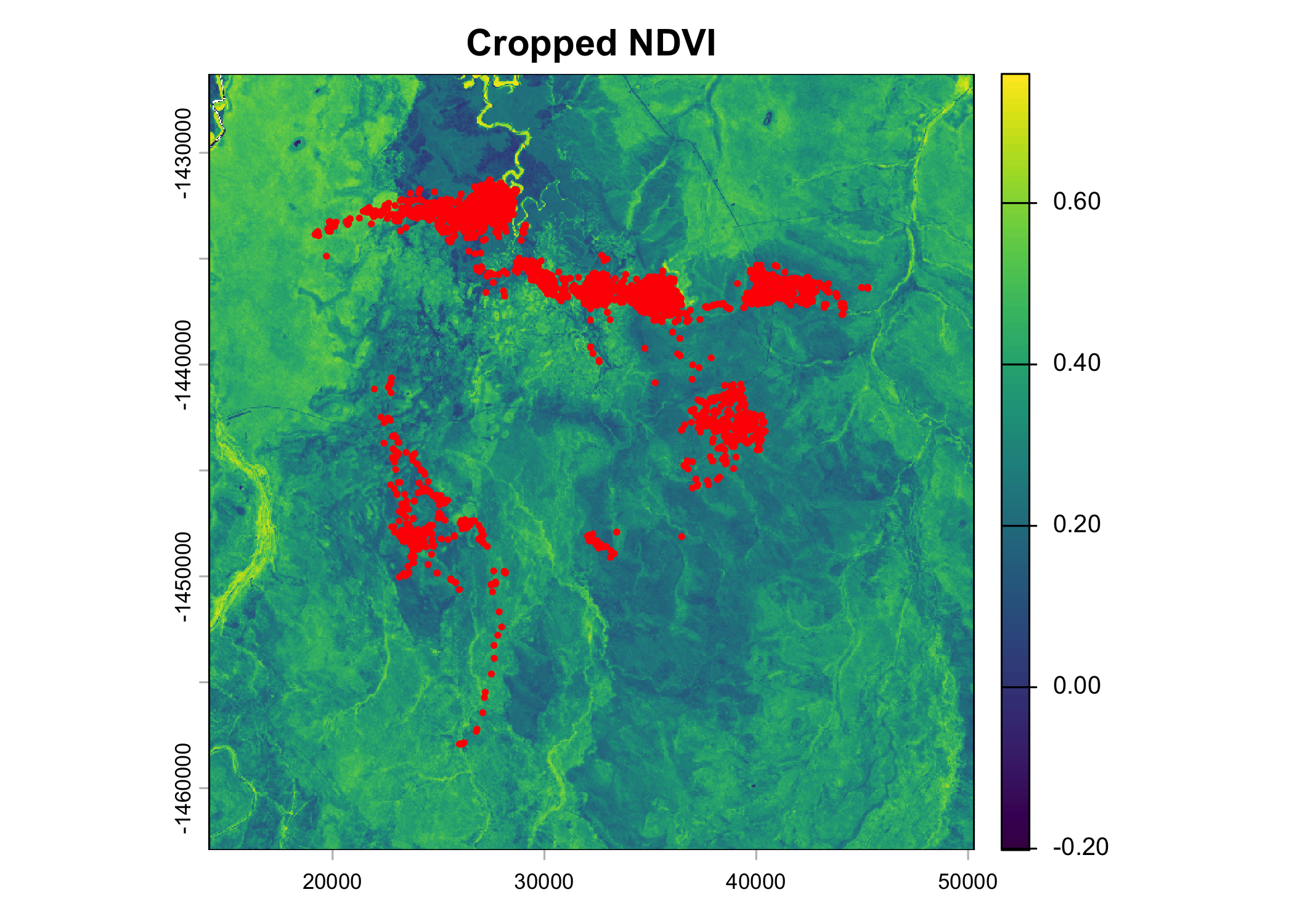

Create dataframes of the covariate values

spatial_covs_cropped_df <- as.data.frame(spatial_covs_cropped, xy = T)

spatial_covs_cropped_df_long <- spatial_covs_cropped_df %>% 
  pivot_longer(cols = -c(x, y), names_to = "covariate", values_to = "value") 

spatial_covs_cropped_df_long %>% 
  ggplot(aes(x = value)) +
  geom_histogram() +
  facet_wrap(~covariate, scales = "free") +
  theme_bw()

`stat_bin()` using `bins = 30`. Pick better value `binwidth`.

Warning: Removed 271 rows containing non-finite outside the scale range
(`stat_bin()`).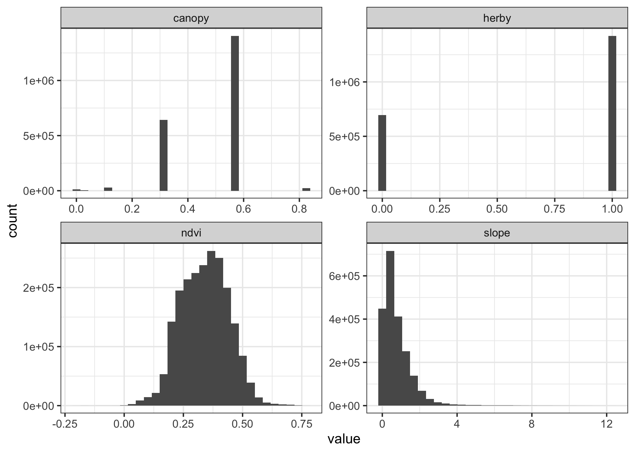

spatial_covs_summary <- spatial_covs_cropped_df_long %>% drop_na() %>%
  group_by(covariate) %>%
  summarise(n = n(),
            mean = mean(value),
            q025 = quantile(value, 0.025),
            q25 = quantile(value, 0.25),
            median = quantile(value, 0.5),
            q75 = quantile(value, 0.75),
            q975 = quantile(value, 0.975)
  )

Extract covariate values at the end of each step

buffalo_id_steps <- buffalo_id_steps %>% 
  extract_covariates(covariates = spatial_covs_cropped, where = "end")

head(buffalo_id_steps)

Prepare data for extracting covariate information

buffalo_id_steps <- buffalo_id_steps %>% 
  mutate(t1_ = lubridate::with_tz(buffalo_id_steps$t1_, tzone = "Australia/Darwin"),
         t2_ = lubridate::with_tz(buffalo_id_steps$t2_, tzone = "Australia/Darwin"))

buffalo_id_steps <- buffalo_id_steps %>%
  mutate(x1 = x1_, x2 = x2_, 
         y1 = y1_, y2 = y2_, 
         t1 = t1_, 
         t1_rounded = round_date(t1_, "hour"), 
         hour_t1 = hour(t1_rounded),
         t2 = t2_, 
         t2_rounded = round_date(t2_, "hour"), 
         hour_t2 = hour(t2_rounded),
         hour_t2 = ifelse(hour_t2 == 0, 24, hour_t2),
         yday = yday(t1_),
         year = year(t1_), 
         month = month(t1_),
         sl = sl_, 
         log_sl = log(sl_), 
         ta = ta_, 
         cos_ta = cos(ta_))

head(buffalo_id_steps) 

Hourly movement behaviour and selection of covariates

Here we bin the trajectories into the hours of the day, and calculate the mean, and quantiles for the step lengths and four habitat covariates. This is a similar approach to in Forrest et al. (2025) and Forrest et al. (2026), where we used this approach to assess temporal dynamics as an exploratory step, but also as a validation step by assessing whether the simulated trajectories had also learned the temporally dynamic behaviour.

Observed buffalo data

buffalo_hourly_habitat <- 
  buffalo_id_steps %>% dplyr::group_by(hour_t2) %>% 
  summarise(n = n(),

            # step lengths
            step_length_mean = mean(sl_),
            step_length_q025 = quantile(sl_, 0.025),
            step_length_q25 = quantile(sl_, 0.25),
            step_length_median = quantile(sl_, 0.5),
            step_length_q75 = quantile(sl_, 0.75),
            step_length_q975 = quantile(sl_, 0.975),

            # ndvi
            ndvi_mean = mean(ndvi),
            ndvi_q025 = quantile(ndvi, 0.025),
            ndvi_q25 = quantile(ndvi, 0.25),
            ndvi_median = median(ndvi),
            ndvi_q75 = quantile(ndvi, 0.75),
            ndvi_q975 = quantile(ndvi, 0.975),

            # herby
            herby_mean = mean(herby),
            herby_q025 = quantile(herby, 0.025),
            herby_q25 = quantile(herby, 0.25),
            herby_median = median(herby),
            herby_q75 = quantile(herby, 0.75),
            herby_q975 = quantile(herby, 0.975),

            # canopy cover
            canopy_mean = mean(canopy),
            canopy_q025 = quantile(canopy, 0.025),
            canopy_q25 = quantile(canopy, 0.25),
            canopy_median = median(canopy),
            canopy_q75 = quantile(canopy, 0.75),
            canopy_q975 = quantile(canopy, 0.975),
            
            # slope
            slope_mean = mean(slope),
            slope_q025 = quantile(slope, 0.025),
            slope_q25 = quantile(slope, 0.25),
            slope_median = median(slope),
            slope_q75 = quantile(slope, 0.75),
            slope_q975 = quantile(slope, 0.975)
            
            ) %>% ungroup()

head(buffalo_hourly_habitat)

Lengthen the dataframe

buffalo_hourly_habitat_long <- buffalo_hourly_habitat %>%
  pivot_longer(cols = !c(hour_t2), names_to = "variable", values_to = "value") %>% 
  filter(!variable == "n")

head(buffalo_hourly_habitat_long)

Set plotting parameters

# set plotting parameters here that will change in each plot

# path
path_linewidth <- 0.5
path_alpha <- 0.1
path_95_alpha <- 1

# ribbon
ribbon_95_alpha <- 0.25
ribbon_50_alpha <- 0.5

Loop over each variable to create a plot

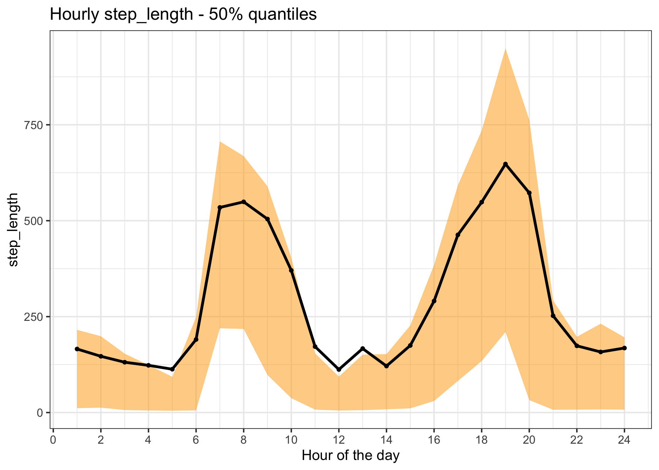
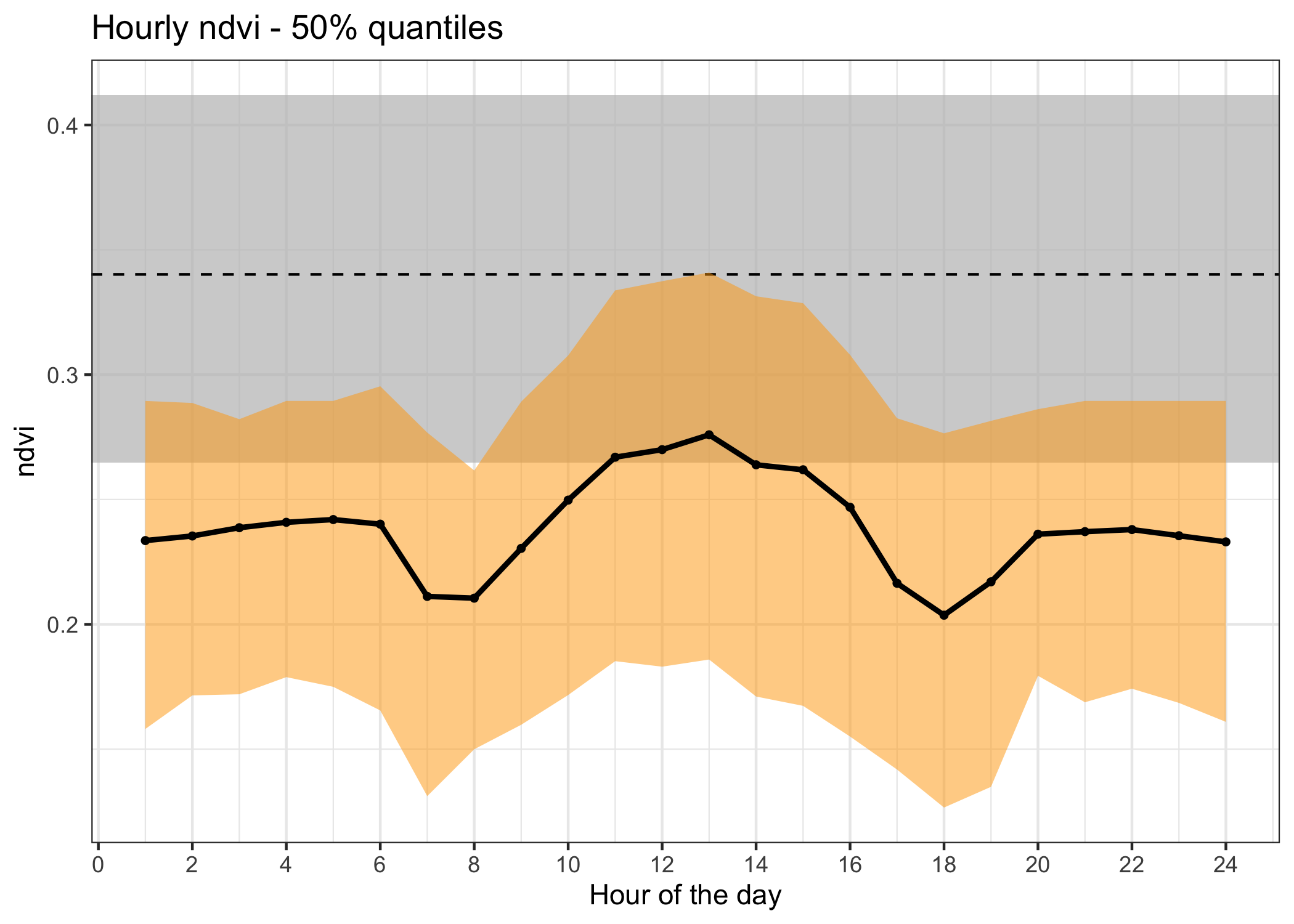
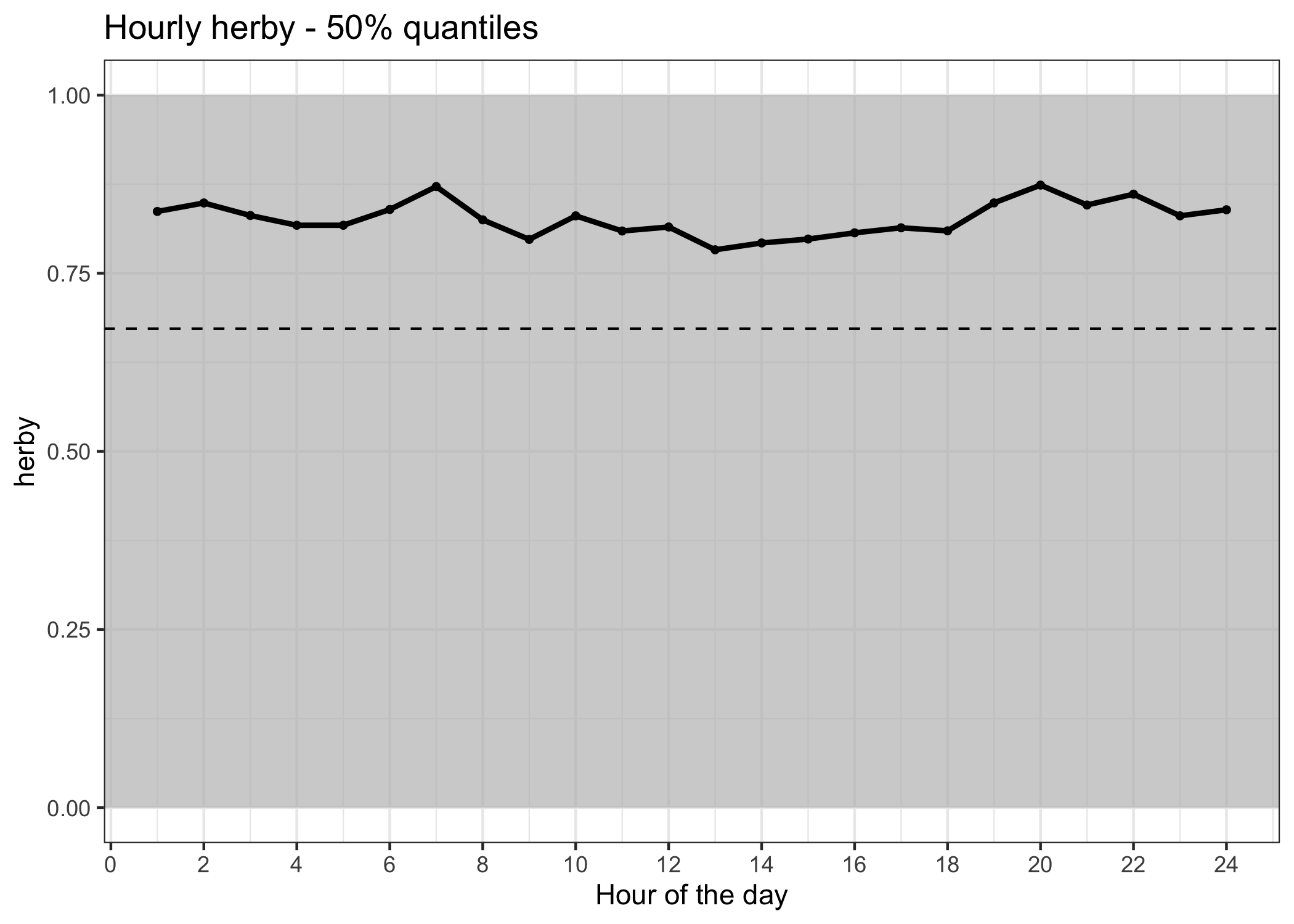
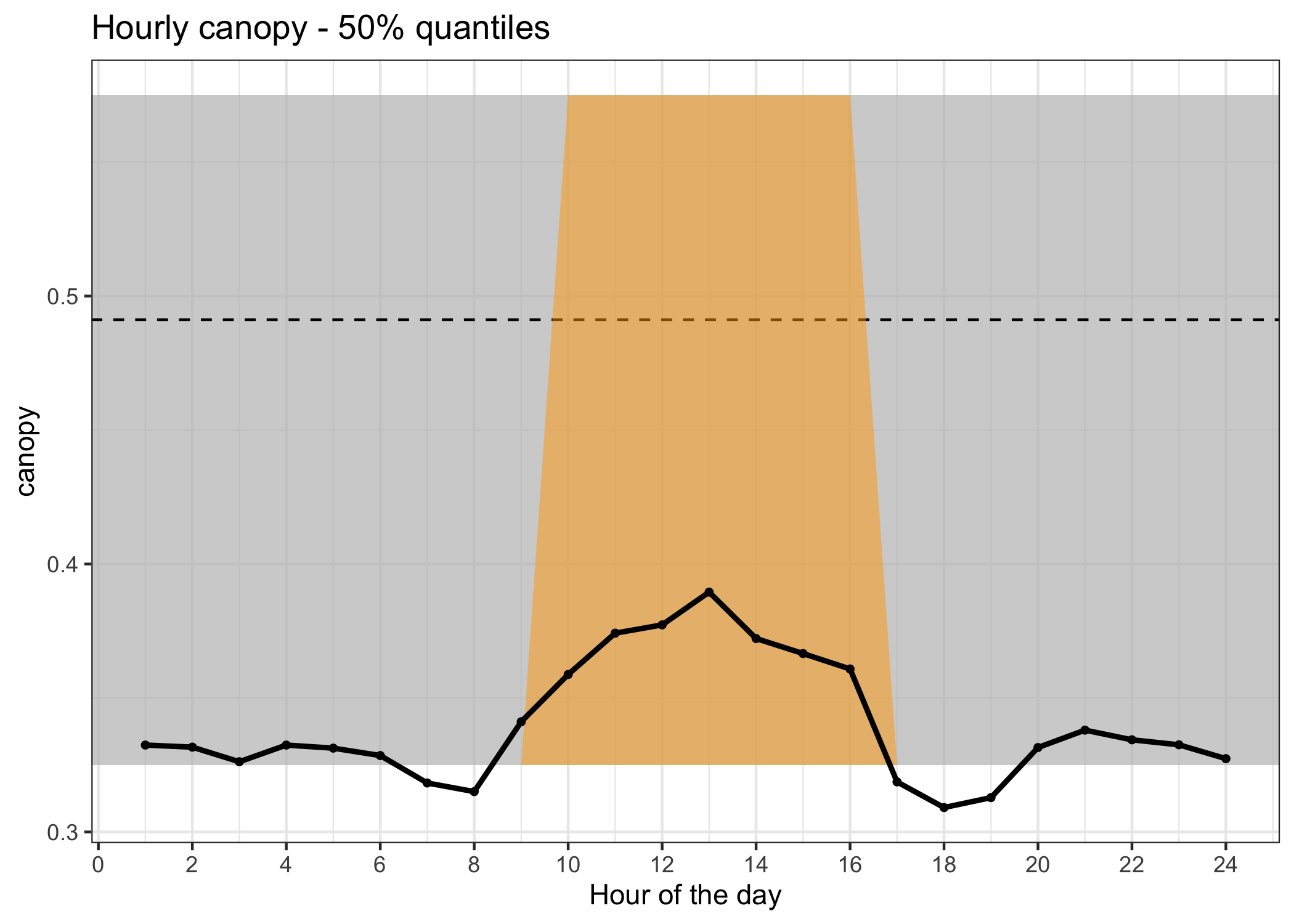
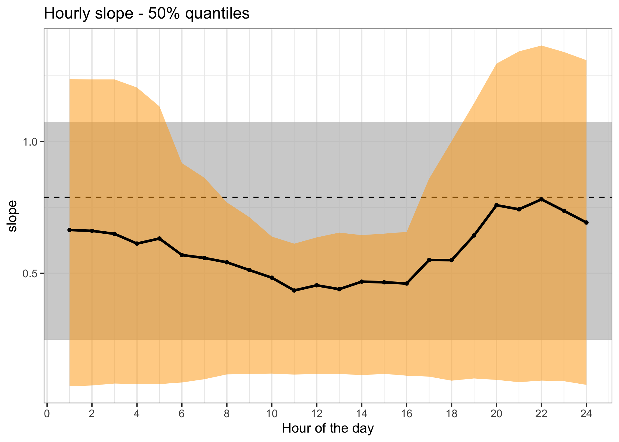
As we have some categorical (canopy cover) and binary variables (herbaceous vegetation), we use the mean for the line, rather than the median. Having categorical and binary variables also explains why some of the ribbons look weird, as the quantile doesn’t change across the day, or jump to a different level (as in the observed ribbon for canopy cover).

In these plots, the grey ribbon represents the 50% quantiles of the covariate values across the landscape (i.e., the background availability), and the dashed line represents the mean value across the landscape. The black line represents the mean value of the covariate at the end of each step, binned by hour of the day, with the orange ribbon representing the 50% quantiles of the covariate values at the end of each step at each hour.

# variables <- unique(buffalo_hourly_habitat_long$variable)

# variables to loop over
variables <- c("step_length", "ndvi", "herby", "canopy", "slope")

for(i in 1:length(variables)){
  
  # Filter data for the current variable
  var_data <- buffalo_hourly_habitat_long %>% 
    filter(str_detect(variable, variables[i]))
  
  # Extract specific quantiles for ribbons
  var_summary <- buffalo_hourly_habitat %>% 
    select(hour_t2, 
           mean = !!paste0(variables[i], "_mean"),
           q025 = !!paste0(variables[i], "_q025"), 
           q25 = !!paste0(variables[i], "_q25"),
           median = !!paste0(variables[i], "_median"),
           q75 = !!paste0(variables[i], "_q75"),
           q975 = !!paste0(variables[i], "_q975"))
  
  spatial_covs_summary_cov <- spatial_covs_summary %>% filter(covariate == variables[i])
  
  plot <- ggplot(data = var_summary) +
    
    # background
    geom_rect(xmin = -Inf, xmax = Inf, 
              ymin = spatial_covs_summary_cov$q25, ymax = spatial_covs_summary_cov$q75, 
              fill = "grey", alpha = 0.05) +
    geom_hline(yintercept = spatial_covs_summary_cov$mean, linetype = "dashed", colour = "black", size = 0.5) +
    
    # ribbons
    # 95% ribbon
    # geom_ribbon(aes(x = hour_t2,
    #                 ymin = q025,
    #                 ymax = q975),
    #             alpha = ribbon_95_alpha, fill = "orange") +
    
    # 50% ribbon
    geom_ribbon(aes(x = hour_t2, 
                    ymin = q25,
                    ymax = q75),
                alpha = ribbon_50_alpha, fill = "orange") +
    
    # lines
    geom_line(aes(x = hour_t2, y = mean), colour = "black", size = 1) +
    geom_point(aes(x = hour_t2, y = mean), colour = "black", size = 1) +
    
    scale_x_continuous(breaks = seq(0, 24, by = 2)) +
    coord_cartesian(expand = TRUE) +
    labs(x = "Hour of the day",
         y = variables[i],
         title = paste0("Hourly ", variables[i], " - 50% quantiles")) +
    theme_bw()
  
  print(plot)

  ggsave(paste0("outputs/exploratory_temporal_dynamics/buffalo_hourly_", variables[i], ".png"),
         plot = plot,
         width = 150, height = 100, units = "mm", dpi = 600)
  
}

Warning: Using `size` aesthetic for lines was deprecated in ggplot2 3.4.0.
ℹ Please use `linewidth` instead.

Warning in geom_rect(xmin = -Inf, xmax = Inf, ymin = spatial_covs_summary_cov$q25, : Ignoring empty aesthetics: `ymin` and `ymax`.
Ignoring empty aesthetics: `ymin` and `ymax`.

References

Forrest, Scott W, Dan Pagendam, Michael Bode, et al. 2025. “Predicting fine‐scale distributions and emergent spatiotemporal patterns from temporally dynamic step selection simulations.” Ecography 2025 (February). https://doi.org/10.1111/ecog.07421.

Forrest, Scott W, Dan Pagendam, Conor Hassan, et al. 2026. “Predicting animal movement with deepSSF : A deep learning step selection framework.” Methods in Ecology and Evolution 17 (February): 371–91. https://doi.org/10.1111/2041-210x.70136.