Comparing SSF and deepSSF Predictions

In this script we are comparing the nezt-step ahead predictions of the SSF (with and without temporal dynamics) and deepSSF models. We are comparing the probabilities of movement, habitat selection and next-step selection, and how they change throughout time.
By comparing the predictions of each process across the entire tracking period or for each hour of the day, we can critically evaluate the covariates that are used by the models and allow for model refinement.
As we expected, the deepSSF models outperformed the SSF models on the in-sample data, which was particularly the case for when the model was trained with Sentinel-2 spectral bands and slope as the spatial covariates (deepSSF S2). The performance dropped for out-of-sample data for all models (including SSFs), and the deepSSF trained with the derived covariates (NDVI, canopy cover, herbaceous vegetation and slope) performed worse than the SSF models, and was only marginally better than a null model, which bears some evidence of overfitting. However, the deepSSF S2 model, trained on `raw’ Sentinel-2 layers rather than derived quantities, retained greater accuracy than all other approaches for out-of-sample data, suggesting that these inputs contain more information that is relevant to buffalo movement and habitat selection than derived quantities like NDVI and slope.
Loading packages
Step selection function probabilities
SSF models fitted with and without temporal dynamics
Code
uniform_prob <- 1/(101*101) # uniform probability for each cell

focal_id <- 2005

n_train <- 0.8
n_val <- 0.1
n_test <- 0.1

# create vector of GPS data filenames
validation_ssf <- list.files(path = "outputs/next_step_validation", pattern = "next_step_probs_ssf_80-10-10_id")
validation_ids <- substr(validation_ssf, 32, 35)

# import data
validation_ssf_list <- vector(mode = "list", length = length(validation_ssf))

for(i in 1:length(validation_ssf)){
  validation_ssf_list[[i]] <-  read_csv(paste("outputs/next_step_validation/",
                                             validation_ssf[[i]],
                                             sep = ""))

  # validation_ssf_list[i]$id <- validation_ids[i]
  attr(validation_ssf_list[[i]]$t_, "tzone") <- "Australia/Queensland"
  attr(validation_ssf_list[[i]]$t2_, "tzone") <- "Australia/Queensland"

  print(sum(is.na(validation_ssf_list[[i]]$prob_next_step_ssf_0p)))

}
[1] 1Code
[1] 10100Determine times for train/val/test splits
Code
# The training data were the first 80%, the validation data were the next 10% and the test were final 10%
train_samples <- nrow(validation_ssf_all) * 0.8
val_test_samples <- nrow(validation_ssf_all) * 0.1

# For plotting
train_val_split <- validation_ssf_all[train_samples,]$t_
val_test_split <- validation_ssf_all[train_samples + val_test_samples,]$t_

# For plotting where example locations were taken from
example_location_A <- validation_ssf_all[1011,]$t_
example_location_B <- validation_ssf_all[3970,]$t_
Split the data into train/validate/test
This is to match the splitting of data that was used to train/fit the deepSSF model. There we used an 80/10/10 split, with 80% of the data for training, 10% for validation, and 10% for testing.
We will follow that same split here, although the validation set is specific to deep learning (it is used to assess when to reduce the learning rate and stop training), with the 10% test data to be used for the held-out validation dataset.
Code
training_split <- 0.8 # 80% of the data will be used for fitting the model
validation_split <- 0.1 # 10% of the data will be used for validation (which isn't used here)
test_split <- 0.1 # 10% of the data will be used for testing (model evaluation)

# Calculate the number of samples for each split
n_samples <- nrow(validation_ssf_all)

n_train <- floor(training_split * n_samples)
n_val <- floor(validation_split * n_samples)
n_test <- n_samples - n_train - n_val  # Ensure they sum to total number of samples

# Print the number of samples in each split
cat("Number of training samples:   ", n_train, "\n")
Number of training samples: 8080 Number of validation samples: 1010 Number of testing samples: 1010 Code
# Get the start and end indices for each split
train_end <- floor(training_split * n_samples)
val_end <- floor((training_split + validation_split) * n_samples)

# Generate indices for each split
train_indices <- 1:train_end
val_indices <- (train_end + 1):val_end
test_indices <- (val_end + 1):n_samples

# Create a new column in the data frame to indicate the dataset
validation_ssf_all <- validation_ssf_all %>% mutate(dataset = NA)

# Add which type of dataset the location should be assigned to
validation_ssf_all$dataset[train_indices] <- "train"
validation_ssf_all$dataset[val_indices] <- "val"
validation_ssf_all$dataset[test_indices] <- "test"

# Timeline of buffalo data
validation_ssf_all %>% ggplot(aes(x = t_, y = factor(dataset), colour = factor(dataset))) +
  geom_point(alpha = 0.1) +
  scale_y_discrete("Buffalo ID") +
  scale_x_datetime("Date") +
  scale_colour_viridis_d() +
  theme_bw() +
  theme(legend.position = "none")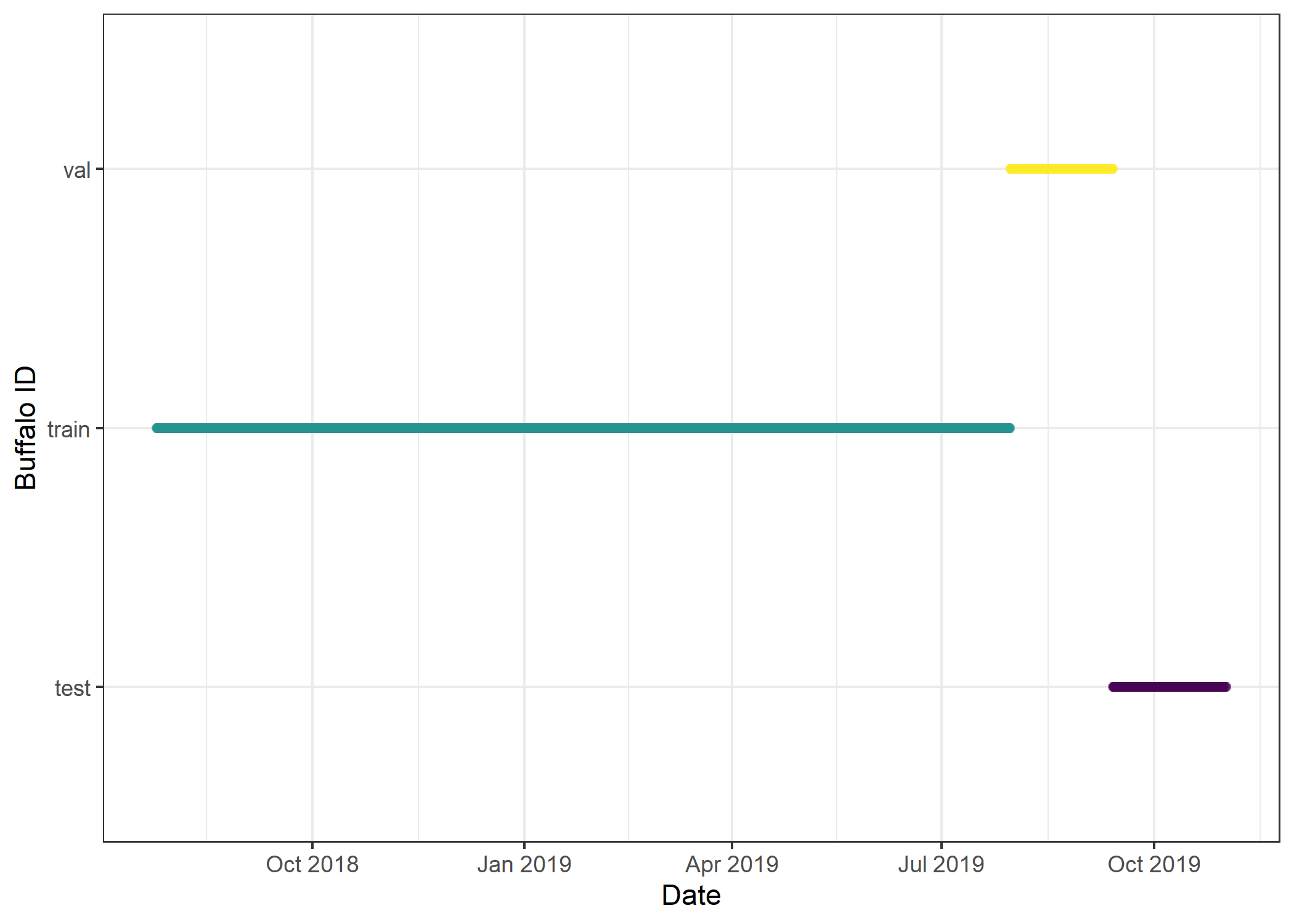
Lengthening data frames to stack together for plotting
Code
validation_ssf_move <- validation_ssf_all %>%
  dplyr::select(dataset, id, x_, y_, t_, x2_, y2_, hour_t1, yday_t1, contains("prob_movement")) %>%
  pivot_longer(cols = contains("movement"),
               names_to = "full_name",
               values_to = "value") %>%
  mutate(
    is_scaled = grepl("_scaled$", full_name),
    model = gsub("prob_movement_", "", full_name) %>% gsub("_scaled$", "", .),
    probability = ifelse(is_scaled, "move_scaled", "move"),
    .after = "full_name"
  ) %>%
  select(-is_scaled)

validation_ssf_habitat <- validation_ssf_all %>%
  dplyr::select(dataset, id, x_, y_, t_, x2_, y2_, hour_t1, yday_t1, contains("prob_habitat")) %>%
  pivot_longer(cols = contains("habitat"),
               names_to = "full_name",
               values_to = "value") %>%
  mutate(
    is_scaled = grepl("_scaled$", full_name),
    model = gsub("prob_habitat_", "", full_name) %>% gsub("_scaled$", "", .),
    probability = ifelse(is_scaled, "habitat_scaled", "habitat"),
    .after = "full_name"
  ) %>%
  select(-is_scaled)

validation_ssf_next_step <- validation_ssf_all %>%
  dplyr::select(dataset, id, x_, y_, t_, x2_, y2_, hour_t1, yday_t1, contains("prob_next_step")) %>%
  pivot_longer(cols = contains("next_step"),
               names_to = "full_name",
               values_to = "value") %>%
  mutate(
    is_scaled = grepl("_scaled$", full_name),
    model = gsub("prob_next_step_", "", full_name) %>% gsub("_scaled$", "", .),
    probability = ifelse(is_scaled, "next_step_scaled", "next_step"),
    .after = "full_name"
  ) %>%
  select(-is_scaled)

validation_ssf_long <- bind_rows(validation_ssf_move,
                                 validation_ssf_habitat,
                                 validation_ssf_next_step)

head(validation_ssf_long)
deepSSF probabilities
Code
New names:
Rows: 10103 Columns: 48
── Column specification
──────────────────────────────────────────────────────── Delimiter: "," dbl
(46): ...1, x_, y_, id, x1_, y1_, x2_, y2_, x2_cent, y2_cent, t_diff, h... dttm
(2): t_, t2_
ℹ Use `spec()` to retrieve the full column specification for this data. ℹ
Specify the column types or set `show_col_types = FALSE` to quiet this message.
• `` -> `...1`
Code
attr(validation_deepssf_all$t_, "tzone") <- "Australia/Queensland"
attr(validation_deepssf_all$t2_, "tzone") <- "Australia/Queensland"

# Create a new column in the data frame to indicate the dataset
validation_deepssf_all <- validation_deepssf_all %>% mutate(dataset = NA)

# Add which type of dataset the location should be assigned to
validation_deepssf_all$dataset[train_indices] <- "train"
validation_deepssf_all$dataset[val_indices] <- "val"
validation_deepssf_all$dataset[test_indices] <- "test"
Lengthening data frames to stack together for plotting
Code
validation_deepssf_long <- validation_deepssf_all %>%
  dplyr::select(dataset, id, x_, y_, t_, x2_, y2_, hour_t1, yday_t1, contains("probs")) %>%
  pivot_longer(cols = contains("probs"),
               names_to = "full_name",
               values_to = "value") %>%
  mutate(model = "deepSSF",
         probability = gsub("_probs", "", full_name),
         .after = "full_name")
deepSSF Sentinel 2 probabilities
Code
validation_deepssf_s2 <- "Python/outputs/model_training_S2/id2005_scalar_movement_9_2025-05-08/deepSSF_validation_id2005_n10103.csv"
validation_ids <- 2005

validation_deepssf_s2_all <- read_csv(validation_deepssf_s2)

attr(validation_deepssf_s2_all$t_, "tzone") <- "Australia/Queensland"
attr(validation_deepssf_s2_all$t2_, "tzone") <- "Australia/Queensland"

# Create a new column in the data frame to indicate the dataset
validation_deepssf_s2_all <- validation_deepssf_s2_all %>% mutate(dataset = NA)

# Add which type of dataset the location should be assigned to
validation_deepssf_s2_all$dataset[train_indices] <- "train"
validation_deepssf_s2_all$dataset[val_indices] <- "val"
validation_deepssf_s2_all$dataset[test_indices] <- "test"
Lengthening data frames to stack together for plotting
Code
validation_deepssf_s2_long <- validation_deepssf_s2_all %>%
  dplyr::select(dataset, id, x_, y_, t_, x2_, y2_, hour_t1, yday_t1, contains("probs")) %>%
  pivot_longer(cols = contains("probs"),
               names_to = "full_name",
               values_to = "value") %>%
  mutate(model = "deepSSF_S2",
         probability = gsub("_probs", "", full_name),
         .after = "full_name")
Combine the lengthened data frames
Calculate average probability and proportion above uniform probability
Code
# calculate the proportion of probabilities above and below the uniform probability
validation_all_summaries <- validation_all_long %>%
  group_by(dataset, probability, model) %>%
  summarise(
    average_prob = mean(value, na.rm = T),
    sd_prob = sd(value, na.rm = T),
    se_prob = sd(value, na.rm = T)/sqrt(n()),
    proportion_above_uniform_prob = sum(value > uniform_prob, na.rm = T)/n(),
    proportion_below_uniform_prob = sum(value < uniform_prob, na.rm = T)/n()) %>%
  ungroup()
`summarise()` has grouped output by 'dataset', 'probability'. You can override
using the `.groups` argument.Prepare data frame for plotting
Code
Prepare sliding window
The predicted probabilities are very noisy, so we apply some smoothing by using a sliding window (rolling mean).
We first need a function to calculate the summary statistics for each window.
Code
window_summary <- function(data) {
  summarise(data,
            average_time = mean(t1_, na.rm = T),
            average_prob = mean(value, na.rm = T),
            q025 = quantile(value, probs = 0.025, na.rm = T),
            q25 = quantile(value, probs = 0.25, na.rm = T),
            q50 = quantile(value, probs = 0.5, na.rm = T),
            q75 = quantile(value, probs = 0.75, na.rm = T),
            q975 = quantile(value, probs = 0.975, na.rm = T)
            )
}
All IDs
Code
window_width <- 15 # number of days in each window - should be odd
# how many observations before and after the current observation
before_after <- (window_width - 1) / 2

# ensure that the data is sorted by time (while respecting the id and model grouping)
validation_all_long <- validation_all_long %>%
  mutate(t1_ = t_) %>%
  group_by(id, model, probability) %>%
  arrange(t1_)

# apply the sliding window function
validation_all_sliding_period <- validation_all_long %>%
  group_by(id, model, probability) %>%
  slide_period_dfr(
    validation_all_long$t1_,
    # specify that we want to split by days (and slide across at daily intervals)
    "day",
    # our window function (calculates mean and quantiles for each window)
    window_summary,
    # how many days before and after the current observation we want to include in the window
    .before = before_after,
    .after = before_after
)

validation_all_long <- validation_all_long %>% ungroup()
validation_all_sliding_period <- validation_all_sliding_period %>% ungroup()

head(validation_all_sliding_period, 10)
We can see from the function above that we have the average time, average probability, and quantiles for each overlapping window, for each model and probability surface (habitat, movement and next-step).
Habitat selection across the tracking period
All models
The solid coloured lines show the average probability for the focal individual that the model was fitted to, and the shaded ribbon is the 50% quantile (there is high variability between probability values, so for clarity we omitted the 95% quantiles). The thin coloured lines are the average probability values for 12 individuals that the model was not fitted to, and are therefore out-of-sample validation data. The dashed coloured lines are the mean values for each model for all of the out-of-sample individuals.
We also show the ‘null’ probability, i.e. if the selection was completely random, which is just the probability divided equally between all cells.
Code
# if there were uniform probabilities (i.e. no selection)
uniform_prob <- 1/(101*101)

ribbon_50_alpha <- 0.1
primary_linewidth <- 0.5
OOS_mean_linewidth <- 0.5
secondary_linewidth <- 0.04

ggplot() +

  # dashed lines containing the SSF probabilities (for zooming into in the paper)
  # geom_hline(yintercept = 0.6e-4, alpha = 0.25, linetype = "dashed", linewidth = 0.25) +
  # geom_hline(yintercept = 1.5e-4, alpha = 0.25, linetype = "dashed", linewidth = 0.25) +

  # dashed lines for train/val/test
  geom_vline(xintercept = train_val_split, linetype = "dashed", linewidth = 0.5) +
  geom_vline(xintercept = val_test_split, linetype = "dashed", linewidth = 0.5) +

  # dashed lines for the example locations
  geom_vline(xintercept = example_location_A, linetype = "dashed", linewidth = 0.5, colour = "grey") +
  geom_vline(xintercept = example_location_B, linetype = "dashed", linewidth = 0.5, colour = "grey") +

  # in sample 50% ribbon
  geom_ribbon(data = validation_all_sliding_period %>%
                filter(probability == "habitat"),
              aes(x = average_time,
                  ymin = q25,
                  ymax = q75,
                  fill = model,
                  group = interaction(id, model)),
              alpha = ribbon_50_alpha) +

  # # quantile line
  # geom_line(data = validation_all_sliding_period %>%
  #             filter(probability == "habitat"),
  #           aes(x = average_time,
  #               y = q975,
  #               colour = model,
  #               group = interaction(id, model)),
  #           linewidth = secondary_linewidth, linetype = "dashed") +

  # in sample mean line
  geom_line(data = validation_all_sliding_period %>%
              filter(probability == "habitat" &
                       !model == "deepSSF_S2 "),
            aes(x = average_time,
                y = average_prob,
                colour = model,
                group = interaction(id, model)),
            linewidth = primary_linewidth) +

  # dashed line for the null probability
  geom_hline(yintercept = uniform_prob, linetype = "dashed", linewidth = 0.5) +

  scale_fill_manual(name = "Model",
                     values = c("#E25834", "#000000", "#0096B5", "#26185F"),
                    labels = c("deepSSF", "deepSSF S2", "iSSF", "iSSF 2p")) +

  scale_color_manual(name = "Model",
                     values = c("#E25834", "#000000", "#0096B5", "#26185F"),
                    labels = c("deepSSF", "deepSSF S2", "iSSF", "iSSF 2p")) +

  # scale_y_continuous("Probability value") +
  scale_y_log10("Habitat selection",
                labels = scales::label_number()) +
  scale_x_datetime("Date") +
  ggtitle("Rolling mean habitat selection probability") +
  theme_bw() +
  theme(legend.position = "bottom",
    axis.text.x = element_text(angle = 30, hjust = 1))
Median
Code
ggplot() +

  # dashed lines containing the SSF probabilities (for zooming into in the paper)
  # geom_hline(yintercept = 0.6e-4, alpha = 0.25, linetype = "dashed", linewidth = 0.25) +
  # geom_hline(yintercept = 1.5e-4, alpha = 0.25, linetype = "dashed", linewidth = 0.25) +

  # dashed lines for train/val/test
  geom_vline(xintercept = train_val_split, linetype = "dashed", linewidth = 0.5) +
  geom_vline(xintercept = val_test_split, linetype = "dashed", linewidth = 0.5) +

  # in sample 50% ribbon
  geom_ribbon(data = validation_all_sliding_period %>%
                filter(probability == "habitat" &
                       !model == "deepSSF_S2 "),
              aes(x = average_time,
                  ymin = q25,
                  ymax = q75,
                  fill = model,
                  group = interaction(id, model)),
              alpha = ribbon_50_alpha) +

  # in sample mean line
  geom_line(data = validation_all_sliding_period %>%
              filter(probability == "habitat" &
                       !model == "deepSSF_S2 "),
            aes(x = average_time,
                y = q50,
                colour = model,
                group = interaction(id, model)),
            linewidth = primary_linewidth) +

  # dashed line for the null probability
  geom_hline(yintercept = uniform_prob, linetype = "dashed", linewidth = 0.5) +

  scale_fill_manual(name = "Model",
                     values = c("#E25834", "#000000", "#0096B5", "#26185F"),
                    labels = c("deepSSF", "deepSSF S2", "SSF", "SSF 2p")) +

  scale_color_manual(name = "Model",
                     values = c("#E25834", "#000000", "#0096B5", "#26185F"),
                    labels = c("deepSSF", "deepSSF S2", "SSF", "SSF 2p")) +

  # scale_y_continuous("Probability value") +
  scale_y_log10("Habitat selection",
                labels = scales::label_number()) +
  ggtitle("Rolling median habitat selection probability") +
  scale_x_datetime("Date") +
  theme_bw() +
  theme(legend.position = "bottom",
    axis.text.x = element_text(angle = 30, hjust = 1))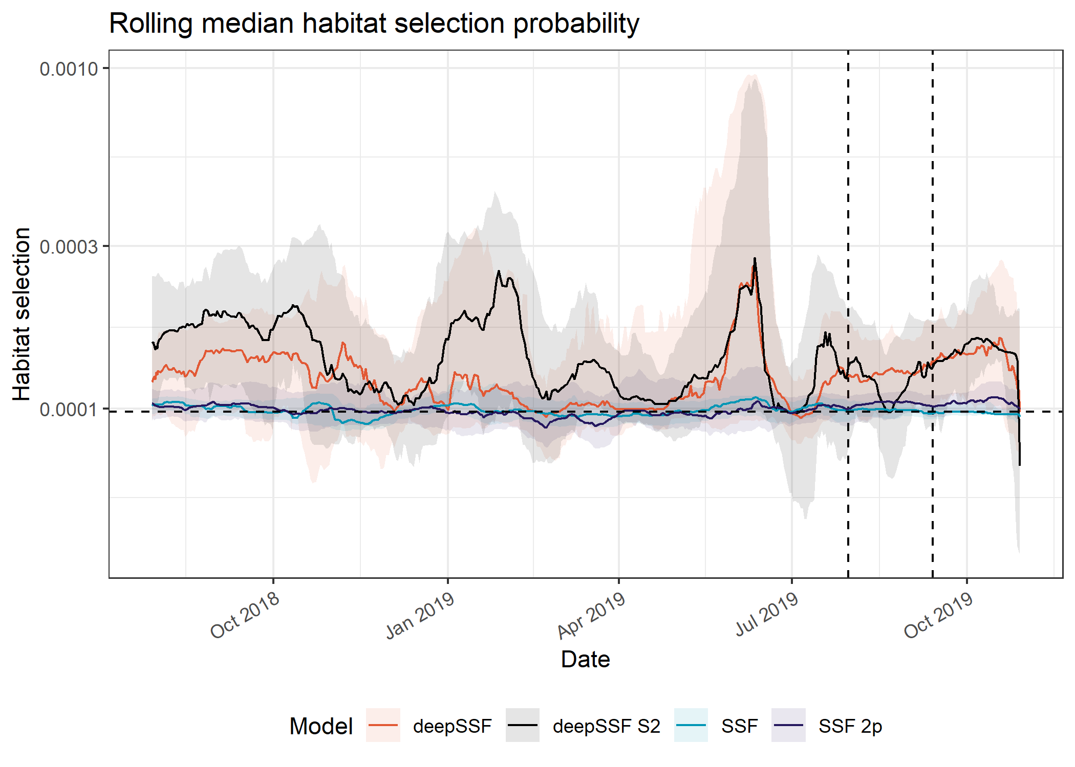
Density of probabilities
Code
lower_truncation_vals <- validation_all_long %>%
  group_by(probability) %>% summarise(
    q01 = quantile(value, probs = 0.01, na.rm = T),
    q99 = quantile(value, probs = 0.99, na.rm = T))

lower_habitat <- lower_truncation_vals %>% filter(probability == "habitat") %>% pull(q01)
upper_habitat <- lower_truncation_vals %>% filter(probability == "habitat") %>% pull(q99)
Plot density of probabilities
Code
# To reverse the factor levels for model
validation_all_long <- validation_all_long %>%
  mutate(model_F = factor(model,
                        levels = c("deepSSF", "deepSSF_S2", "ssf_0p", "ssf_2p"),
                        labels = c("deepSSF", "deepSSF S2", "iSSF", "iSSF 2p")))

ggplot() +

  geom_vline(xintercept = uniform_prob, linetype = "dashed", linewidth = 0.5) +

  geom_density_ridges(data = validation_all_long %>%
                 filter(probability == "habitat" & value > lower_habitat & value < upper_habitat),
               aes(x = value, y = model_F, fill = model_F, colour = model_F),
               alpha = 0.15, scale = 3, quantile_lines = TRUE, quantiles = 2) +

  scale_fill_manual(name = "Model",
                     values = c("#E25834", "#000000", "#0096B5", "#26185F"),
                    labels = c("deepSSF", "deepSSF S2", "iSSF", "iSSF 2p")) +

  scale_color_manual(name = "Model",
                     values = c("#E25834", "#000000", "#0096B5", "#26185F"),
                    labels = c("deepSSF", "deepSSF S2", "iSSF", "iSSF 2p")) +

  scale_x_log10("Habitat selection",
                labels = scales::label_number()) +
  scale_y_discrete("") +
  theme_bw() +
  theme(legend.position = "none",
        plot.margin = margin(t = 0.1, r = 0.65, b = 0.15, l = 0, unit = "cm"))
Picking joint bandwidth of 0.0227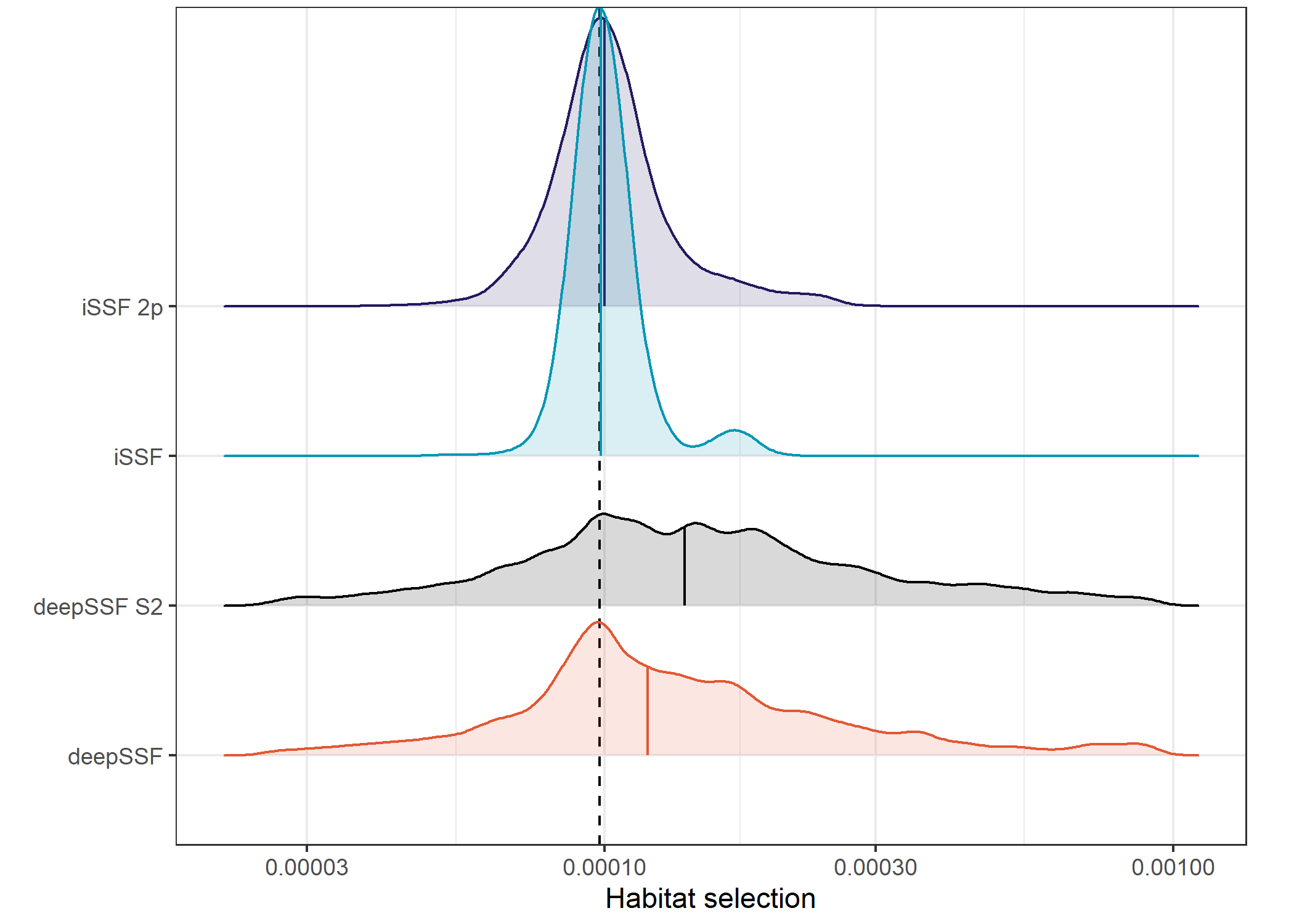
Code
Picking joint bandwidth of 0.0227The first thing to note is difference in magnitude between the deepSSF and the SSF predictions. The deepSSF predicted probabilities are often much higher, but can also be much lower, suggesting that the deepSSF models are more ‘confident’.
The deepSSF and deepSSF S2 models both performed particularly well between December 2018 and July 2019, (wet-season and early dry-season), although only the deepSSF S2 model performs well outside of this period (for most of the dry season). This suggests that the derived covariates may lack information that is relevant to buffalo during this period, such as a representation of water.
The higher performance of the deepSSF S2 predictions is also echoed in the out-of-sample predictions, which are generally quite a lot higher than the other models.
deepSSF models
Code
ggplot() +

  # # dashed lines containing the SSF probabilities (for zooming into in the paper)
  # geom_hline(yintercept = 0.6e-4, alpha = 0.25, linetype = "dashed", linewidth = 0.25) +
  # geom_hline(yintercept = 1.5e-4, alpha = 0.25, linetype = "dashed", linewidth = 0.25) +

  # dashed lines for train/val/test
  geom_vline(xintercept = train_val_split, linetype = "dashed", linewidth = 0.25) +
  geom_vline(xintercept = val_test_split, linetype = "dashed", linewidth = 0.25) +

  # in sample 50% ribbon
  geom_ribbon(data = validation_all_sliding_period %>%
                filter(probability == "habitat" &
                       id == focal_id &
                       grepl("deepSSF", model)),
              aes(x = average_time,
                  ymin = q25,
                  ymax = q75,
                  fill = model,
                  group = interaction(id, model)),
              alpha = ribbon_50_alpha) +

  # in sample mean line
  geom_line(data = validation_all_sliding_period %>%
              filter(probability == "habitat" &
                     id == focal_id &
                     grepl("deepSSF", model)),
            aes(x = average_time,
                y = average_prob,
                colour = model,
                group = interaction(id, model)),
            linewidth = primary_linewidth) +

  # dashed line for the null probability
  geom_hline(yintercept = uniform_prob, linetype = "dashed", linewidth = 0.5) +

  scale_fill_manual(name = "Model",
                     values = c("#E25834", "#000000"),
                    labels = c("deepSSF", "deepSSF S2")) +

  scale_color_manual(name = "Model",
                     values = c("#E25834", "#000000"),
                    labels = c("deepSSF", "deepSSF S2")) +

  # scale_y_continuous("Probability value") +
  scale_y_log10("Probability value") +
  scale_x_datetime("Date") +
  theme_bw() +
  theme(legend.position = "bottom",
    axis.text.x = element_text(angle = 30, hjust = 1))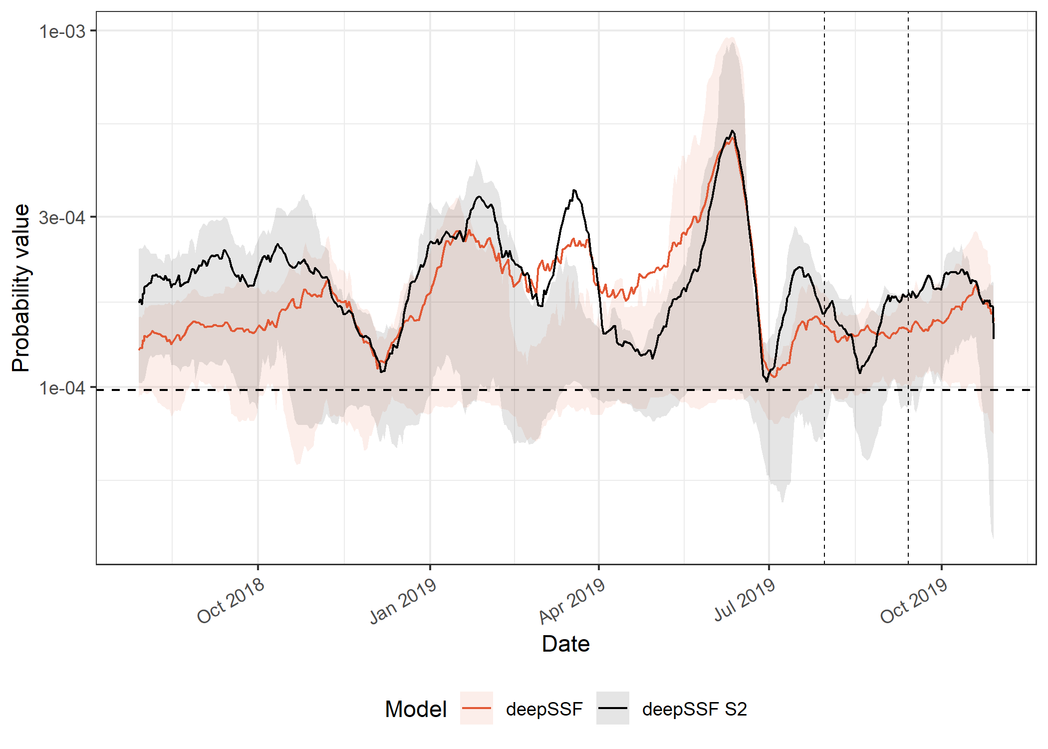
SSF models
Code
ggplot() +

  # dashed lines for train/val/test
  geom_vline(xintercept = train_val_split, linetype = "dashed", linewidth = 0.25) +
  geom_vline(xintercept = val_test_split, linetype = "dashed", linewidth = 0.25) +

  # in sample 50% ribbon
  geom_ribbon(data = validation_all_sliding_period %>%
                filter(probability == "habitat",
                       id == focal_id,
                       !grepl("deepSSF", model)),
              aes(x = average_time,
                  ymin = q25,
                  ymax = q75,
                  fill = model,
                  group = interaction(id, model)),
              alpha = ribbon_50_alpha) +

  # in sample mean line
  geom_line(data = validation_all_sliding_period %>%
              filter(probability == "habitat",
                     id == focal_id,
                     !grepl("deepSSF", model)),
            aes(x = average_time,
                y = average_prob,
                colour = model,
                group = interaction(id, model)),
            linewidth = primary_linewidth) +

  # dashed line for the null probability
  geom_hline(yintercept = uniform_prob, linetype = "dashed", linewidth = 0.5) +

  scale_fill_manual(name = "Model",
                     values = c("#0096B5", "#26185F"),
                    labels = c("SSF", "SSF 2p")) +

  scale_color_manual(name = "Model",
                     values = c("#0096B5", "#26185F"),
                    labels = c("SSF", "SSF 2p")) +

  scale_y_continuous("Probability value",
                     position = "right",
                     labels = function(x) format(x, scientific = TRUE)) +

  scale_x_datetime("Date") +
  coord_cartesian(ylim = c(0.6e-4, 1.5e-4)) +
  theme_bw() +
  theme(legend.position = "bottom",
    axis.text.x = element_text(angle = 30, hjust = 1))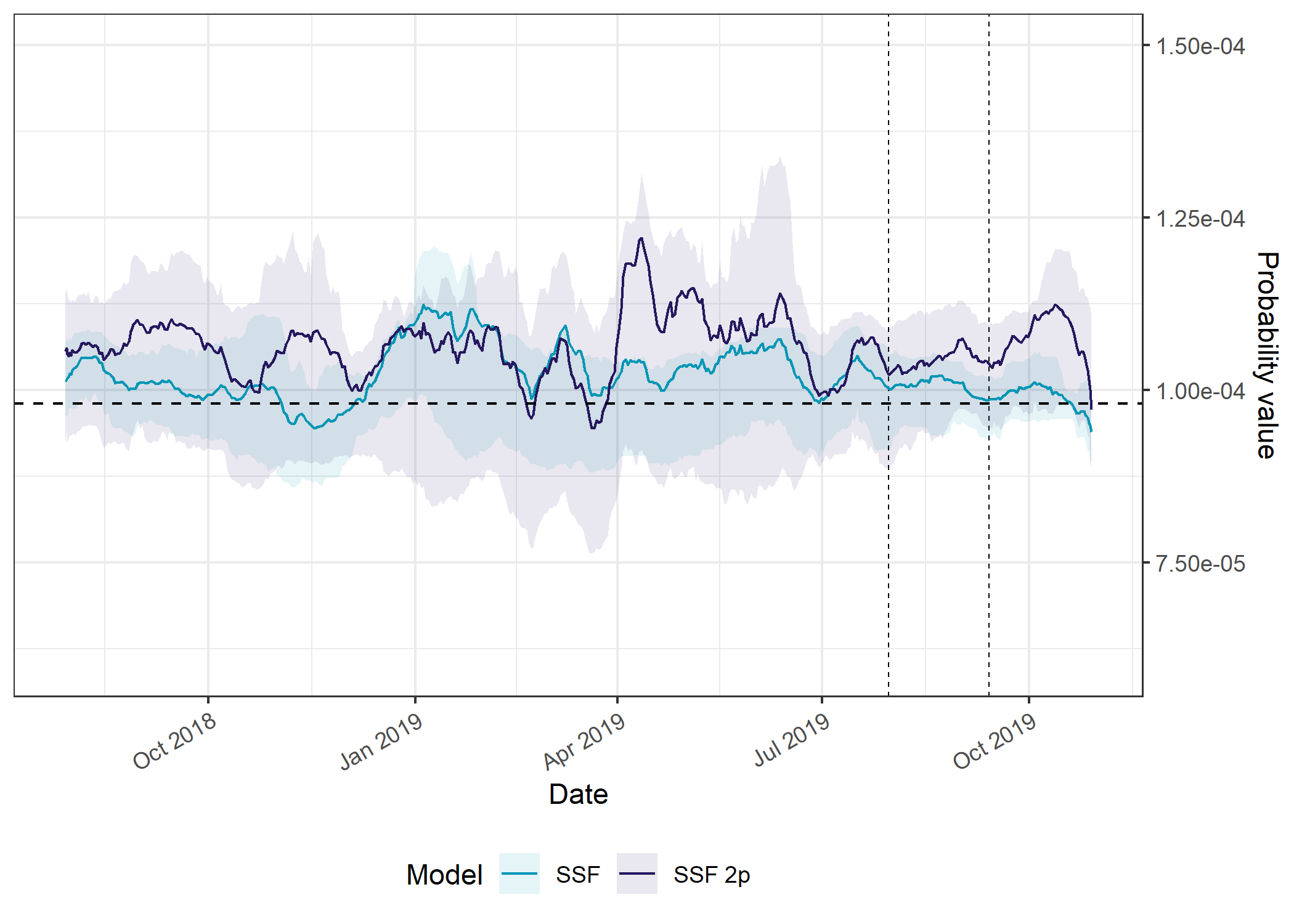
There isn’t a clear seasonal trend with the SSF predictions, but in general the models do better than the null model, although the out-of-sample predictions vary around the null model.
Movement probability across the tracking period
All models
Mean probability
Code
ggplot() +

  # # dashed lines containing the SSF probabilities
  # geom_hline(yintercept = 0.6e-4, alpha = 0.25, linetype = "dashed", linewidth = 0.25) +
  # geom_hline(yintercept = 1.5e-4, alpha = 0.25, linetype = "dashed", linewidth = 0.25) +

  # dashed lines for train/val/test
  geom_vline(xintercept = train_val_split, linetype = "dashed", linewidth = 0.5) +
  geom_vline(xintercept = val_test_split, linetype = "dashed", linewidth = 0.5) +

  # in sample 50% ribbon
  geom_ribbon(data = validation_all_sliding_period %>%
                filter(probability == "move" &
                       id == focal_id),
              aes(x = average_time,
                  ymin = q25,
                  ymax = q75,
                  fill = model,
                  group = interaction(id, model)),
              alpha = ribbon_50_alpha) +

  # in sample mean line
  geom_line(data = validation_all_sliding_period %>%
              filter(probability == "move" &
                     id == focal_id),
            aes(x = average_time,
                y = average_prob,
                colour = model,
                group = interaction(id, model)),
            linewidth = primary_linewidth) +

  # dashed line for the null probability
  geom_hline(yintercept = uniform_prob, linetype = "dashed", linewidth = 0.5) +

  scale_fill_manual(name = "Model",
                     values = c("#E25834", "#000000", "#0096B5", "#26185F"),
                    labels = c("deepSSF", "deepSSF S2", "SSF", "SSF 2p")) +

  scale_color_manual(name = "Model",
                     values = c("#E25834", "#000000", "#0096B5", "#26185F"),
                    labels = c("deepSSF", "deepSSF S2", "SSF", "SSF 2p")) +

  # scale_y_continuous("Probability value") +
  scale_y_log10("Movement probability") +
  scale_x_datetime("Date") +
  ggtitle("Rolling mean movement probability") +
  theme_bw() +
  theme(legend.position = "bottom",
    axis.text.x = element_text(angle = 30, hjust = 1))
Density of probabilities
Plot density of probabilities
Code
# To reverse the factor levels for model
validation_all_long <- validation_all_long %>%
  mutate(model_F = factor(model,
                        levels = c("deepSSF", "deepSSF_S2", "ssf_0p", "ssf_2p"),
                        labels = c("deepSSF", "deepSSF S2", "iSSF", "iSSF 2p")))

ggplot() +

  geom_vline(xintercept = uniform_prob, linetype = "dashed", linewidth = 0.5) +

  geom_density_ridges(data = validation_all_long %>%
                 filter(probability == "move" & value > lower_habitat & value < upper_habitat),
               aes(x = value, y = model_F, fill = model_F, colour = model_F),
               alpha = 0.15, scale = 2, quantile_lines = TRUE, quantiles = 2) +

  scale_fill_manual(name = "Model",
                     values = c("#E25834", "#000000", "#0096B5", "#26185F"),
                    labels = c("deepSSF", "deepSSF S2", "iSSF", "iSSF 2p")) +

  scale_color_manual(name = "Model",
                     values = c("#E25834", "#000000", "#0096B5", "#26185F"),
                    labels = c("deepSSF", "deepSSF S2", "iSSF", "iSSF 2p")) +

  scale_x_log10("Movement probability",
                labels = scales::label_number()) +
  scale_y_discrete("") +
  theme_bw() +
  theme(legend.position = "none",
        plot.margin = margin(t = 0.1, r = 0.65, b = 0.15, l = 0, unit = "cm"))
Picking joint bandwidth of 0.0735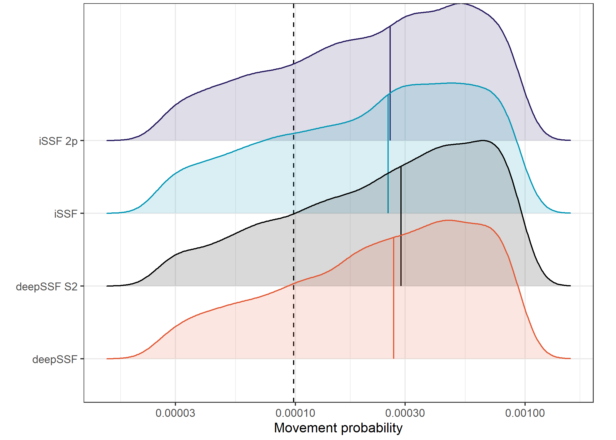
Code
Picking joint bandwidth of 0.0735Median
Code
ggplot() +

  # # dashed lines containing the SSF probabilities
  # geom_hline(yintercept = 0.6e-4, alpha = 0.25, linetype = "dashed", linewidth = 0.25) +
  # geom_hline(yintercept = 1.5e-4, alpha = 0.25, linetype = "dashed", linewidth = 0.25) +

  # dashed lines for train/val/test
  geom_vline(xintercept = train_val_split, linetype = "dashed", linewidth = 0.5) +
  geom_vline(xintercept = val_test_split, linetype = "dashed", linewidth = 0.5) +

  # # in sample 50% ribbon
  geom_ribbon(data = validation_all_sliding_period %>%
                filter(probability == "move" &
                       id == focal_id),
              aes(x = average_time,
                  ymin = q25,
                  ymax = q75,
                  fill = model,
                  group = interaction(id, model)),
              alpha = ribbon_50_alpha) +

  # in sample mean line
  geom_line(data = validation_all_sliding_period %>%
              filter(probability == "move" &
                     id == focal_id),
            aes(x = average_time,
                y = q50,
                colour = model,
                group = interaction(id, model)),
            linewidth = primary_linewidth) +

  # dashed line for the null probability
  geom_hline(yintercept = uniform_prob, linetype = "dashed", linewidth = 0.5) +

  scale_fill_manual(name = "Model",
                     values = c("#E25834", "#000000", "#0096B5", "#26185F"),
                    labels = c("deepSSF", "deepSSF S2", "SSF", "SSF 2p")) +

  scale_color_manual(name = "Model",
                     values = c("#E25834", "#000000", "#0096B5", "#26185F"),
                    labels = c("deepSSF", "deepSSF S2", "SSF", "SSF 2p")) +

  # scale_y_continuous("Probability value") +
  scale_y_log10("Movement probability") +
  scale_x_datetime("Date") +
  ggtitle("Rolling median movement probability") +
  theme_bw() +
  theme(legend.position = "bottom",
    axis.text.x = element_text(angle = 30, hjust = 1))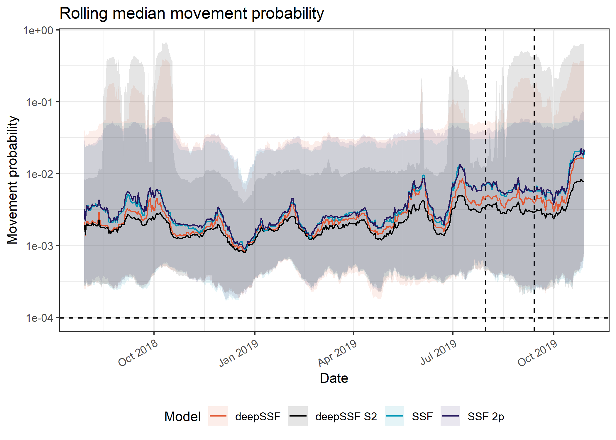
The movement probabilities for the deepSSF models are much higher than the for the SSF models, which I suspect is mostly due to the mixture of distributions in the deepSSF models. When the buffalo are in a low movement period, there can be very high probability in the few cells close to the buffalo, which is often accurate (when the predicted probability is 0.2 that means all of the probability mass is shared between only 5 cells. I don’t think the SSF movement kernel has the same flexibility to capture this.
This also comes out very clearly in the hourly predictions, with much higher predicted probabilities during the low movement periods.
deepSSF models
Code
ggplot() +

  # # dashed lines containing the SSF probabilities
  # geom_hline(yintercept = 0, alpha = 0.25, linetype = "dashed", linewidth = 0.25) +
  # geom_hline(yintercept = 9e-3, alpha = 0.25, linetype = "dashed", linewidth = 0.25) +

  # dashed lines for train/val/test
  geom_vline(xintercept = train_val_split, linetype = "dashed", linewidth = 0.25) +
  geom_vline(xintercept = val_test_split, linetype = "dashed", linewidth = 0.25) +

  # in sample 50% ribbon
  geom_ribbon(data = validation_all_sliding_period %>%
                filter(probability == "move" &
                       id == focal_id &
                       grepl("deepSSF", model)),
              aes(x = average_time,
                  ymin = q25,
                  ymax = q75,
                  fill = model,
                  group = interaction(id, model)),
              alpha = ribbon_50_alpha) +

  # in sample mean line
  geom_line(data = validation_all_sliding_period %>%
              filter(probability == "move" &
                     id == focal_id &
                     grepl("deepSSF", model)),
            aes(x = average_time,
                y = average_prob,
                colour = model,
                group = interaction(id, model)),
            linewidth = primary_linewidth) +

  # dashed line for the null probability
  geom_hline(yintercept = uniform_prob, linetype = "dashed", linewidth = 0.5) +

  scale_fill_manual(name = "Model",
                     values = c("#E25834", "#000000"),
                    labels = c("deepSSF", "deepSSF S2")) +

  scale_color_manual(name = "Model",
                     values = c("#E25834", "#000000"),
                    labels = c("deepSSF", "deepSSF S2")) +

  scale_y_continuous("Probability value") +
  scale_x_datetime("Date") +
  theme_bw() +
  theme(legend.position = "bottom",
    axis.text.x = element_text(angle = 30, hjust = 1))
SSF models
Code
ggplot() +

  # dashed lines for train/val/test
  geom_vline(xintercept = train_val_split, linetype = "dashed", linewidth = 0.25) +
  geom_vline(xintercept = val_test_split, linetype = "dashed", linewidth = 0.25) +

  # in sample 50% ribbon
  geom_ribbon(data = validation_all_sliding_period %>%
                filter(probability == "move",
                       id == focal_id,
                       !grepl("deepSSF", model)),
              aes(x = average_time,
                  ymin = q25,
                  ymax = q75,
                  fill = model,
                  group = interaction(id, model)),
              alpha = ribbon_50_alpha) +

  # in sample mean line
  geom_line(data = validation_all_sliding_period %>%
              filter(probability == "move",
                     id == focal_id,
                     !grepl("deepSSF", model)),
            aes(x = average_time,
                y = average_prob,
                colour = model,
                group = interaction(id, model)),
            linewidth = primary_linewidth) +

  # dashed line for the null probability
  geom_hline(yintercept = uniform_prob, linetype = "dashed", linewidth = 0.5) +

  scale_fill_manual(name = "Model",
                     values = c("#0096B5", "#26185F"),
                    labels = c("SSF", "SSF 2p")) +

  scale_color_manual(name = "Model",
                     values = c("#0096B5", "#26185F"),
                    labels = c("SSF", "SSF 2p")) +

    scale_y_continuous("Probability value",
                     position = "right") +

  scale_x_datetime("Date") +
  # coord_cartesian(ylim = c(0, 9e-3)) +
  theme_bw() +
  theme(legend.position = "bottom",
    axis.text.x = element_text(angle = 30, hjust = 1))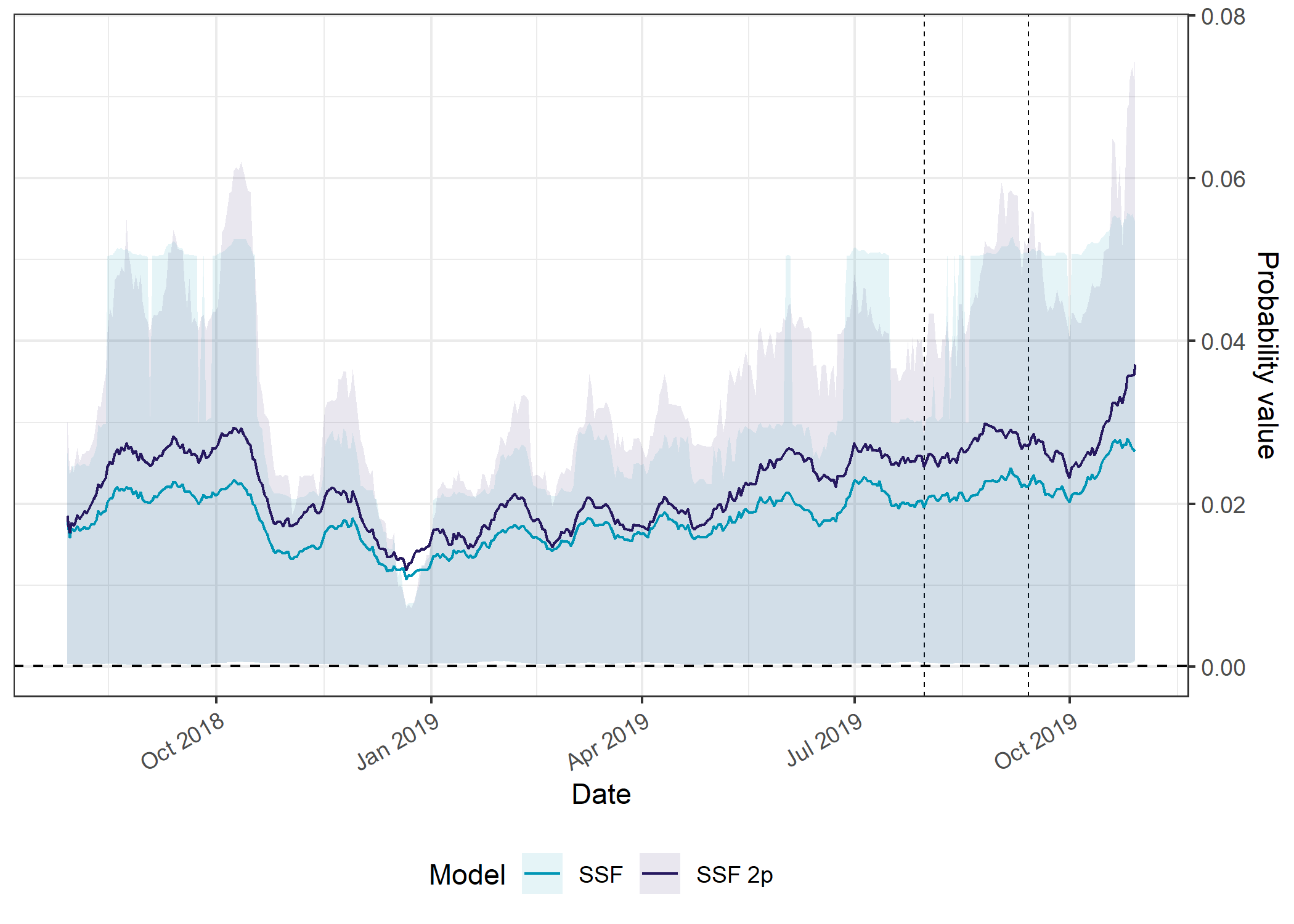
The temporally dynamic models have consistently higher probabilities of movement than the static models, which again is likely due to the concentration of the movement kernel during the low movement periods, where the probability values are distributed across much fewer cells.
Next-step probabilities across the tracking period
The next-step probability values are very similar to the movement probabilities due to the concentration of the probability mass in fewer cells that are closer to the buffalo, whereas the habitat selection probabilities are distributed across all of the local layers, so they’re not actually that informative beyond the movement probabilities.
All models
Code
ggplot() +

  # # dashed lines containing the SSF probability values
  # geom_hline(yintercept = 0.6e-4, alpha = 0.25, linetype = "dashed", linewidth = 0.25) +
  # geom_hline(yintercept = 1.5e-4, alpha = 0.25, linetype = "dashed", linewidth = 0.25) +

  # dashed lines for train/val/test
  geom_vline(xintercept = train_val_split, linetype = "dashed", linewidth = 0.5) +
  geom_vline(xintercept = val_test_split, linetype = "dashed", linewidth = 0.5) +

  # in sample 50% ribbon
  geom_ribbon(data = validation_all_sliding_period %>%
                filter(probability == "next_step" &
                       id == focal_id),
              aes(x = average_time,
                  ymin = q25,
                  ymax = q75,
                  fill = model,
                  group = interaction(id, model)),
              alpha = ribbon_50_alpha) +

  # in sample mean line
  geom_line(data = validation_all_sliding_period %>%
              filter(probability == "next_step" &
                     id == focal_id),
            aes(x = average_time,
                y = average_prob,
                colour = model,
                group = interaction(id, model)),
            linewidth = primary_linewidth) +

  # dashed line for the null probability
  geom_hline(yintercept = uniform_prob, linetype = "dashed", linewidth = 0.5) +

  scale_fill_manual(name = "Model",
                     values = c("#E25834", "#000000", "#0096B5", "#26185F"),
                    labels = c("deepSSF", "deepSSF S2", "SSF", "SSF 2p")) +

  scale_color_manual(name = "Model",
                     values = c("#E25834", "#000000", "#0096B5", "#26185F"),
                    labels = c("deepSSF", "deepSSF S2", "SSF", "SSF 2p")) +

  # scale_y_continuous("Probability value") +
  scale_y_log10("Next-step probability") +
  scale_x_datetime("Date") +
  ggtitle("Rolling mean next-step probability") +
  theme_bw() +
  theme(legend.position = "bottom",
    axis.text.x = element_text(angle = 30, hjust = 1))
Density of probabilities
Plot density of probabilities
Code
# To reverse the factor levels for model
validation_all_long <- validation_all_long %>%
  mutate(model_F = factor(model,
                        levels = c("deepSSF", "deepSSF_S2", "ssf_0p", "ssf_2p"),
                        labels = c("deepSSF", "deepSSF S2", "iSSF", "iSSF 2p")))

ggplot() +

  geom_vline(xintercept = uniform_prob, linetype = "dashed", linewidth = 0.5) +

  geom_density_ridges(data = validation_all_long %>%
                 filter(probability == "next_step" & value > lower_habitat & value < upper_habitat),
               aes(x = value, y = model_F, fill = model_F, colour = model_F),
               alpha = 0.15, scale = 2, quantile_lines = TRUE, quantiles = 2) +

  scale_fill_manual(name = "Model",
                     values = c("#E25834", "#000000", "#0096B5", "#26185F"),
                    labels = c("deepSSF", "deepSSF S2", "iSSF", "iSSF 2p")) +

  scale_color_manual(name = "Model",
                     values = c("#E25834", "#000000", "#0096B5", "#26185F"),
                    labels = c("deepSSF", "deepSSF S2", "iSSF", "iSSF 2p")) +

  scale_x_log10("Next step probability",
                labels = scales::label_number()) +
  scale_y_discrete("") +
  theme_bw() +
  theme(legend.position = "none",
        plot.margin = margin(t = 0.1, r = 0.65, b = 0.15, l = 0, unit = "cm"))
Picking joint bandwidth of 0.0746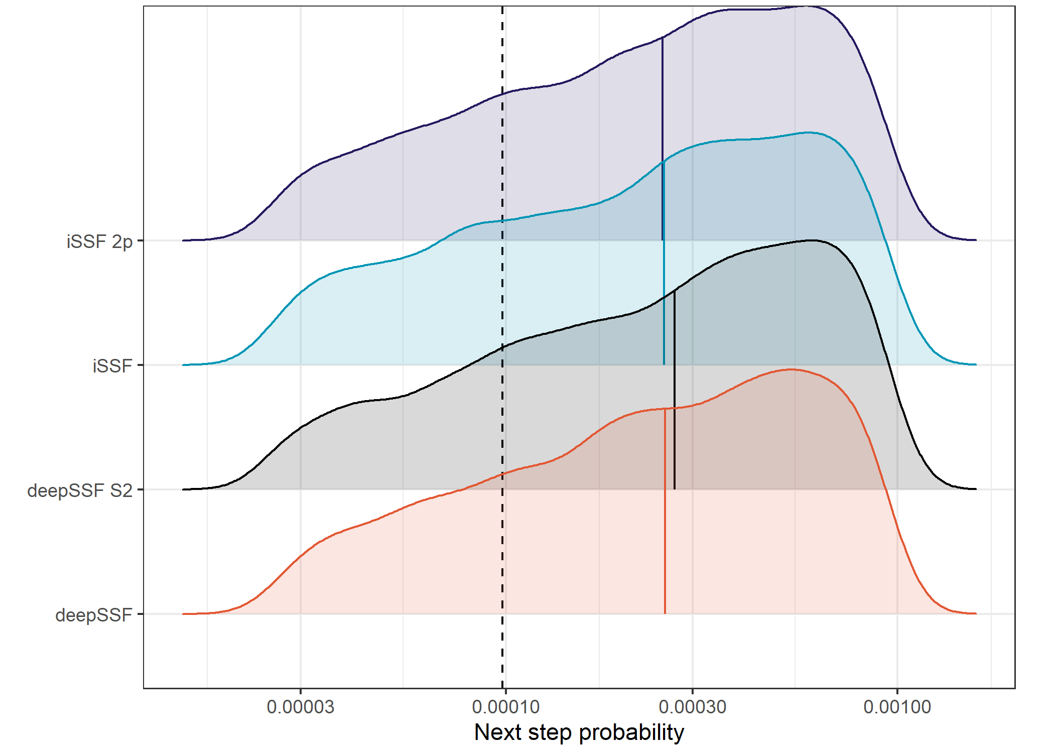
Code
Picking joint bandwidth of 0.0746Median
Code
ggplot() +

  # # dashed lines containing the SSF probabilities
  # geom_hline(yintercept = 0.6e-4, alpha = 0.25, linetype = "dashed", linewidth = 0.25) +
  # geom_hline(yintercept = 1.5e-4, alpha = 0.25, linetype = "dashed", linewidth = 0.25) +

  # dashed lines for train/val/test
  geom_vline(xintercept = train_val_split, linetype = "dashed", linewidth = 0.5) +
  geom_vline(xintercept = val_test_split, linetype = "dashed", linewidth = 0.5) +

  # # in sample 50% ribbon
  geom_ribbon(data = validation_all_sliding_period %>%
                filter(probability == "next_step" &
                       id == focal_id),
              aes(x = average_time,
                  ymin = q25,
                  ymax = q75,
                  fill = model,
                  group = interaction(id, model)),
              alpha = ribbon_50_alpha) +

  # in sample mean line
  geom_line(data = validation_all_sliding_period %>%
              filter(probability == "next_step" &
                     id == focal_id),
            aes(x = average_time,
                y = q50,
                colour = model,
                group = interaction(id, model)),
            linewidth = primary_linewidth) +

  # dashed line for the null probability
  geom_hline(yintercept = uniform_prob, linetype = "dashed", linewidth = 0.5) +

  scale_fill_manual(name = "Model",
                     values = c("#E25834", "#000000", "#0096B5", "#26185F"),
                    labels = c("deepSSF", "deepSSF S2", "SSF", "SSF 2p")) +

  scale_color_manual(name = "Model",
                     values = c("#E25834", "#000000", "#0096B5", "#26185F"),
                    labels = c("deepSSF", "deepSSF S2", "SSF", "SSF 2p")) +

  # scale_y_continuous("Probability value") +
  scale_y_log10("Probability value") +
  scale_x_datetime("Date") +
  ggtitle("Rolling median next-step probability") +
  theme_bw() +
  theme(legend.position = "bottom",
    axis.text.x = element_text(angle = 30, hjust = 1))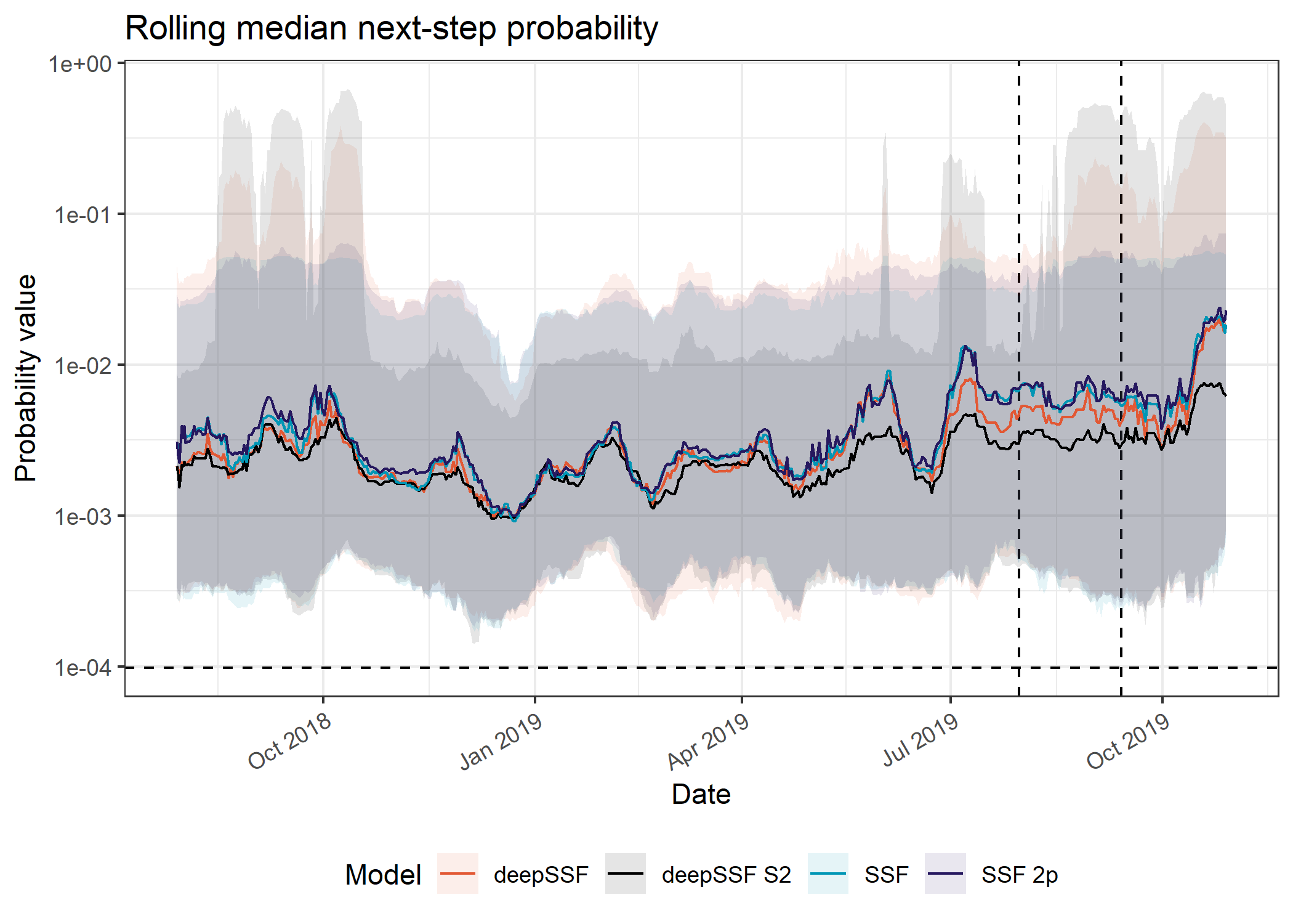
deepSSF models
Code
ggplot() +

  # # dashed lines containing the SSF probability values
  # geom_hline(yintercept = 0, alpha = 0.25, linetype = "dashed", linewidth = 0.25) +
  # geom_hline(yintercept = 9e-3, alpha = 0.25, linetype = "dashed", linewidth = 0.25) +

  # dashed lines for train/val/test
  geom_vline(xintercept = train_val_split, linetype = "dashed", linewidth = 0.25) +
  geom_vline(xintercept = val_test_split, linetype = "dashed", linewidth = 0.25) +

  # in sample 50% ribbon
  geom_ribbon(data = validation_all_sliding_period %>%
                filter(probability == "next_step" &
                       id == focal_id &
                       grepl("deepSSF", model)),
              aes(x = average_time,
                  ymin = q25,
                  ymax = q75,
                  fill = model,
                  group = interaction(id, model)),
              alpha = ribbon_50_alpha) +

  # in sample mean line
  geom_line(data = validation_all_sliding_period %>%
              filter(probability == "next_step" &
                     id == focal_id &
                     grepl("deepSSF", model)),
            aes(x = average_time,
                y = average_prob,
                colour = model,
                group = interaction(id, model)),
            linewidth = primary_linewidth) +

  # dashed line for the null probability
  geom_hline(yintercept = uniform_prob, linetype = "dashed", linewidth = 0.5) +

  scale_fill_manual(name = "Model",
                     values = c("#E25834", "#000000"),
                    labels = c("deepSSF", "deepSSF S2")) +

  scale_color_manual(name = "Model",
                     values = c("#E25834", "#000000"),
                    labels = c("deepSSF", "deepSSF S2")) +

  scale_y_continuous("Probability value") +
  scale_x_datetime("Date") +
  theme_bw() +
  theme(legend.position = "bottom",
    axis.text.x = element_text(angle = 30, hjust = 1))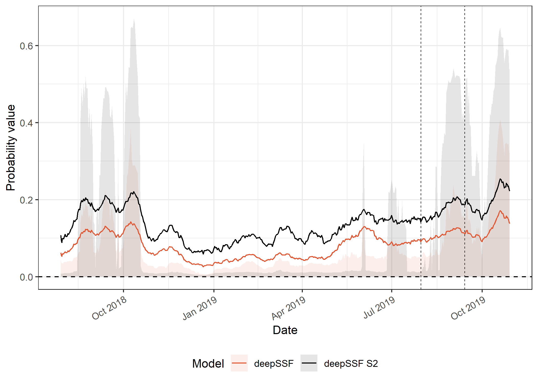
SSF models
Code
ggplot() +

  # dashed lines for train/val/test
  geom_vline(xintercept = train_val_split, linetype = "dashed", linewidth = 0.25) +
  geom_vline(xintercept = val_test_split, linetype = "dashed", linewidth = 0.25) +

  # in sample 50% ribbon
  geom_ribbon(data = validation_all_sliding_period %>%
                filter(probability == "next_step",
                       id == focal_id,
                       !grepl("deepSSF", model)),
              aes(x = average_time,
                  ymin = q25,
                  ymax = q75,
                  fill = model,
                  group = interaction(id, model)),
              alpha = ribbon_50_alpha) +

  # in sample mean line
  geom_line(data = validation_all_sliding_period %>%
              filter(probability == "next_step",
                     id == focal_id,
                     !grepl("deepSSF", model)),
            aes(x = average_time,
                y = average_prob,
                colour = model,
                group = interaction(id, model)),
            linewidth = primary_linewidth) +

  # dashed line for the null probability
  geom_hline(yintercept = uniform_prob, linetype = "dashed", linewidth = 0.5) +

  scale_fill_manual(name = "Model",
                     values = c("#0096B5", "#26185F"),
                    labels = c("SSF", "SSF 2p")) +

  scale_color_manual(name = "Model",
                     values = c("#0096B5", "#26185F"),
                    labels = c("SSF", "SSF 2p")) +

    scale_y_continuous("Probability value",
                     position = "right") +

  scale_x_datetime("Date") +
  # coord_cartesian(ylim = c(0, 9e-3)) +
  theme_bw() +
  theme(legend.position = "bottom",
    axis.text.x = element_text(angle = 30, hjust = 1))
Hourly probabilities
We can also calculate the habitat selection, movement and next-step probabilities for each hour of the day, indicating when the models are accurate (or notr) at different times of the day.
For this we don’t need a sliding window, we will just bin by the hour of the day.
Here we just show the hourly probabilities across the whole tracking period, but we could also split this up into seasons and assess how accurate the models are during the wet and dry seasons.
Code
# grouping by each individual, model and hour of the day
validation_all_quantiles_hourly <- validation_all_long %>%
  filter(hour_t1 < 24) %>%
  group_by(id, model, probability, hour_t1) %>%
  summarise(average_prob = mean(value, na.rm = T),
            sd_prob = sd(value, na.rm = T),
            q025 = quantile(value, probs = 0.025, na.rm = T),
            q25 = quantile(value, probs = 0.25, na.rm = T),
            q50 = quantile(value, probs = 0.5, na.rm = T),
            q75 = quantile(value, probs = 0.75, na.rm = T),
            q975 = quantile(value, probs = 0.975, na.rm = T)
            )
`summarise()` has grouped output by 'id', 'model', 'probability'. You can
override using the `.groups` argument.Habitat selection across the day
All models
Code
ggplot() +

  # dashed lines containing the SSF probabilities
  # geom_hline(yintercept = 0, alpha = 0.25, linetype = "dashed", linewidth = 0.25) +
  # geom_hline(yintercept = 3e-4, alpha = 0.25, linetype = "dashed", linewidth = 0.25) +

  # in sample 50% ribbon
  geom_ribbon(data = validation_all_quantiles_hourly %>%
                filter(probability == "habitat",
                       id == focal_id),
              aes(x = hour_t1,
                  ymin = q25,
                  ymax = q75,
                  fill = model,
                  group = interaction(id, model)),
              alpha = ribbon_50_alpha) +

  # in sample mean line
  geom_line(data = validation_all_quantiles_hourly %>%
              filter(probability == "habitat",
                     id == focal_id),
            aes(x = hour_t1,
                y = average_prob,
                colour = model,
                group = interaction(id, model)),
            linewidth = primary_linewidth) +

  # dashed line for the null probability
  geom_hline(yintercept = uniform_prob, linetype = "dashed", linewidth = 0.25) +

  scale_fill_manual(name = "Model",
                     values = c("#AF3602", "#000000", "#0096B5", "#26185F"),
                    labels = c("deepSSF", "deepSSF S2", "SSF", "SSF 2p")) +

  scale_color_manual(name = "Model",
                     values = c("#AF3602", "#000000", "#0096B5", "#26185F"),
                    labels = c("deepSSF", "deepSSF S2", "SSF", "SSF 2p")) +

  # scale_y_continuous("Probability value") +
  scale_y_log10("Habitat selection",
                labels = scales::label_number()) +
  scale_x_continuous("Hour", breaks = seq(0,24,6)) +
  theme_bw() +
  theme(legend.position = "none")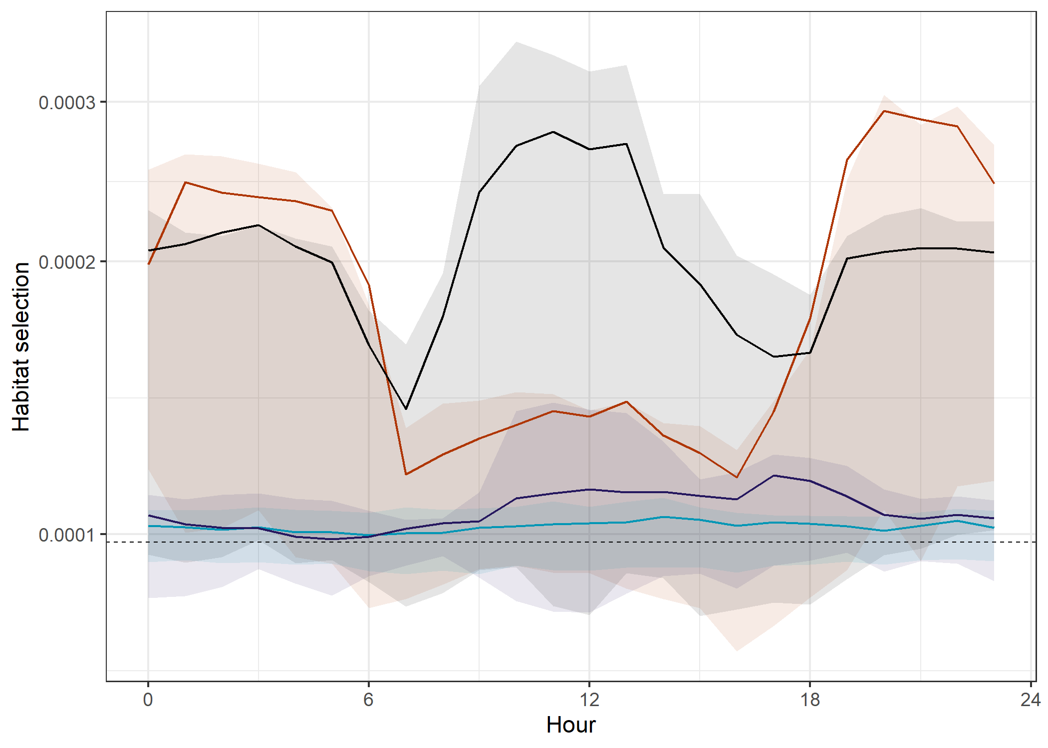
The deepSSF models both predict well in the evening (at least in-sample), but only the deepSSF S2 predicts well during the middle of the day, again suggesting that there is information in the Sentinel-2 layers that isn’t present in the derived covariates.
The out-of-sample predictions are also much higher for the deepSSF S2 model, suggesting that it is better at generalising to new data.
deepSSF models
Code
ggplot() +

  # dashed lines containing the SSF probabilities
  # geom_hline(yintercept = 0.6e-4, alpha = 0.25, linetype = "dashed", linewidth = 0.25) +
  # geom_hline(yintercept = 1.5e-4, alpha = 0.25, linetype = "dashed", linewidth = 0.25) +

  # in sample 50% ribbon
  geom_ribbon(data = validation_all_quantiles_hourly %>%
                filter(probability == "habitat",
                       id == focal_id,
                       grepl("deepSSF", model)),
              aes(x = hour_t1,
                  ymin = q25,
                  ymax = q75,
                  fill = model,
                  group = interaction(id, model)),
              alpha = ribbon_50_alpha) +

  # in sample mean line
  geom_line(data = validation_all_quantiles_hourly %>%
              filter(probability == "habitat",
                     id == focal_id,
                     grepl("deepSSF", model)),
            aes(x = hour_t1,
                y = average_prob,
                colour = model,
                group = interaction(id, model)),
            linewidth = primary_linewidth) +

  # dashed line for the null probability
  geom_hline(yintercept = uniform_prob, linetype = "dashed", linewidth = 0.25) +

  scale_fill_manual(name = "Model",
                     values = c("#E25834", "#000000"),
                    labels = c("deepSSF", "deepSSF S2")) +

  scale_color_manual(name = "Model",
                     values = c("#E25834", "#000000"),
                    labels = c("deepSSF", "deepSSF S2")) +

  # scale_y_continuous("Probability value") +
  scale_y_log10("Probability value") +
  scale_x_continuous("Hour", seq(0,24,6)) +
  # coord_cartesian(ylim = c(0, 4e-4)) +
  theme_bw() +
  theme(legend.position = "bottom")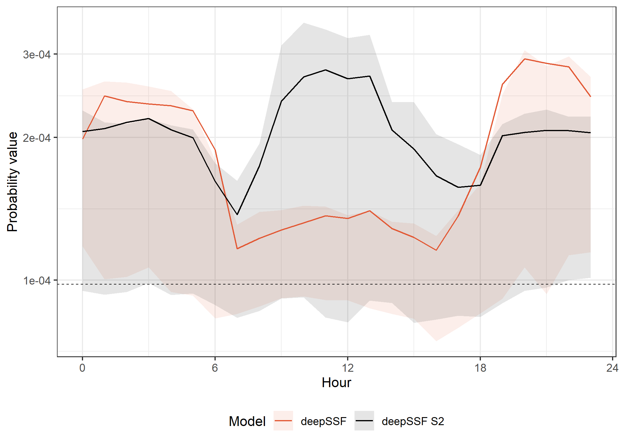
SSF models
Code
ggplot() +

  # in sample 50% ribbon
  geom_ribbon(data = validation_all_quantiles_hourly %>%
                filter(probability == "habitat",
                       id == focal_id,
                       !grepl("deepSSF", model)),
              aes(x = hour_t1,
                  ymin = q25,
                  ymax = q75,
                  fill = model,
                  group = interaction(id, model)),
              alpha = ribbon_50_alpha) +

  # in sample mean line
  geom_line(data = validation_all_quantiles_hourly %>%
              filter(probability == "habitat",
                     id == focal_id,
                     !grepl("deepSSF", model)),
            aes(x = hour_t1,
                y = average_prob,
                colour = model,
                group = interaction(id, model)),
            linewidth = primary_linewidth) +

  # dashed line for the null probability
  geom_hline(yintercept = uniform_prob, linetype = "dashed", linewidth = 0.25) +

  scale_fill_manual(name = "Model",
                     values = c("#0096B5", "#26185F"),
                    labels = c("SSF", "SSF 2p")) +

  scale_color_manual(name = "Model",
                     values = c("#0096B5", "#26185F"),
                    labels = c("SSF", "SSF 2p")) +

  scale_y_continuous("Probability value",
                     # position = "right",
                     labels = function(x) format(x, scientific = TRUE)) +

  scale_x_continuous("Hour", seq(0,24,6)) +
  # coord_cartesian(ylim = c(0.6e-4, 1.5e-4)) +
  theme_bw() +
  theme(legend.position = "bottom")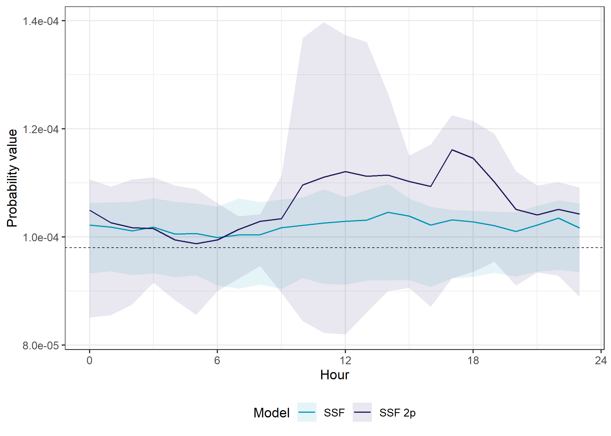
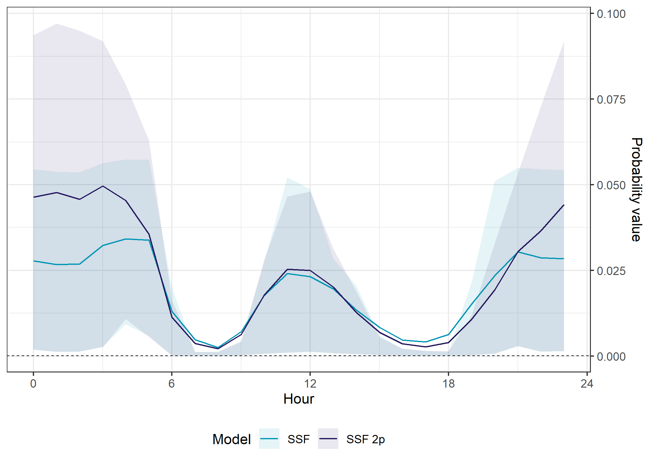
The SSF model with temporal dynamics had higher prediction accuracy than the SSF model without temporal dynamics overall (in- and out-of-sample), but it was more variable throughout the day, and was quite poor between midnight and about 5am.
Movement probability across the day
All models
Code
ggplot() +

  # dashed lines containing the SSF probabilities
  # geom_hline(yintercept = 0, alpha = 0.25, linetype = "dashed", linewidth = 0.25) +
  # geom_hline(yintercept = 3e-4, alpha = 0.25, linetype = "dashed", linewidth = 0.25) +

  # in sample 50% ribbon
  geom_ribbon(data = validation_all_quantiles_hourly %>%
                filter(probability == "move",
                       id == focal_id),
              aes(x = hour_t1,
                  ymin = q25,
                  ymax = q75,
                  fill = model,
                  group = interaction(id, model)),
              alpha = ribbon_50_alpha) +

  # in sample mean line
  geom_line(data = validation_all_quantiles_hourly %>%
              filter(probability == "move",
                     id == focal_id),
            aes(x = hour_t1,
                y = average_prob,
                colour = model,
                group = interaction(id, model)),
            linewidth = 0.35) +

  geom_hline(yintercept = uniform_prob, linetype = "dashed", linewidth = 0.25) +

  scale_fill_manual(name = "Model",
                     values = c("#AF3602", "#000000", "#0096B5", "#000000"),
                    labels = c("deepSSF", "deepSSF S2", "SSF", "SSF 2p")) +

  scale_color_manual(name = "Model",
                     values = c("#AF3602", "#000000", "#0096B5", "#000000"),
                    labels = c("deepSSF", "deepSSF S2", "SSF", "SSF 2p")) +

  # scale_y_continuous("Probability value") +
  scale_y_log10("Probability value") +
  scale_x_continuous("Hour", breaks = seq(0,24,6)) +
  theme_bw() +
  theme(legend.position = "bottom")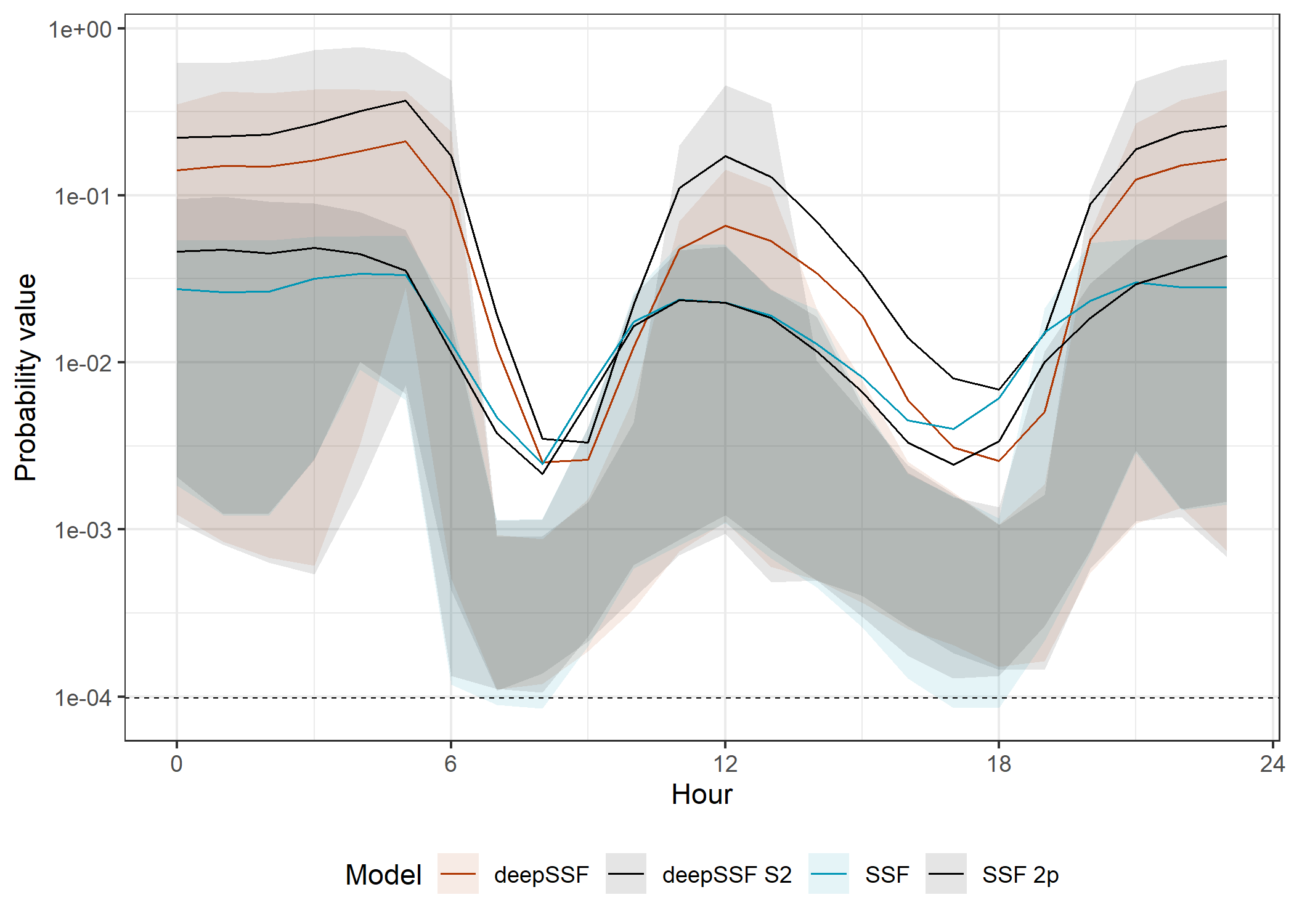
Median
Code
ggplot() +

  # dashed lines containing the SSF probabilities
  # geom_hline(yintercept = 0, alpha = 0.25, linetype = "dashed", linewidth = 0.25) +
  # geom_hline(yintercept = 3e-4, alpha = 0.25, linetype = "dashed", linewidth = 0.25) +

  # in sample 50% ribbon
  geom_ribbon(data = validation_all_quantiles_hourly %>%
                filter(probability == "move",
                       id == focal_id),
              aes(x = hour_t1,
                  ymin = q25,
                  ymax = q75,
                  fill = model,
                  group = interaction(id, model)),
              alpha = ribbon_50_alpha) +

  # in sample mean line
  geom_line(data = validation_all_quantiles_hourly %>%
              filter(probability == "move",
                     id == focal_id),
            aes(x = hour_t1,
                y = q50,
                colour = model,
                group = interaction(id, model)),
            linewidth = 0.35) +

  geom_hline(yintercept = uniform_prob, linetype = "dashed", linewidth = 0.25) +

  scale_fill_manual(name = "Model",
                     values = c("#AF3602", "#000000", "#0096B5", "#000000"),
                    labels = c("deepSSF", "deepSSF S2", "SSF", "SSF 2p")) +

  scale_color_manual(name = "Model",
                     values = c("#AF3602", "#000000", "#0096B5", "#000000"),
                    labels = c("deepSSF", "deepSSF S2", "SSF", "SSF 2p")) +

  # scale_y_continuous("Probability value") +
  scale_y_log10("Probability value") +
  scale_x_continuous("Hour", breaks = seq(0,24,6)) +
  theme_bw() +
  theme(legend.position = "bottom")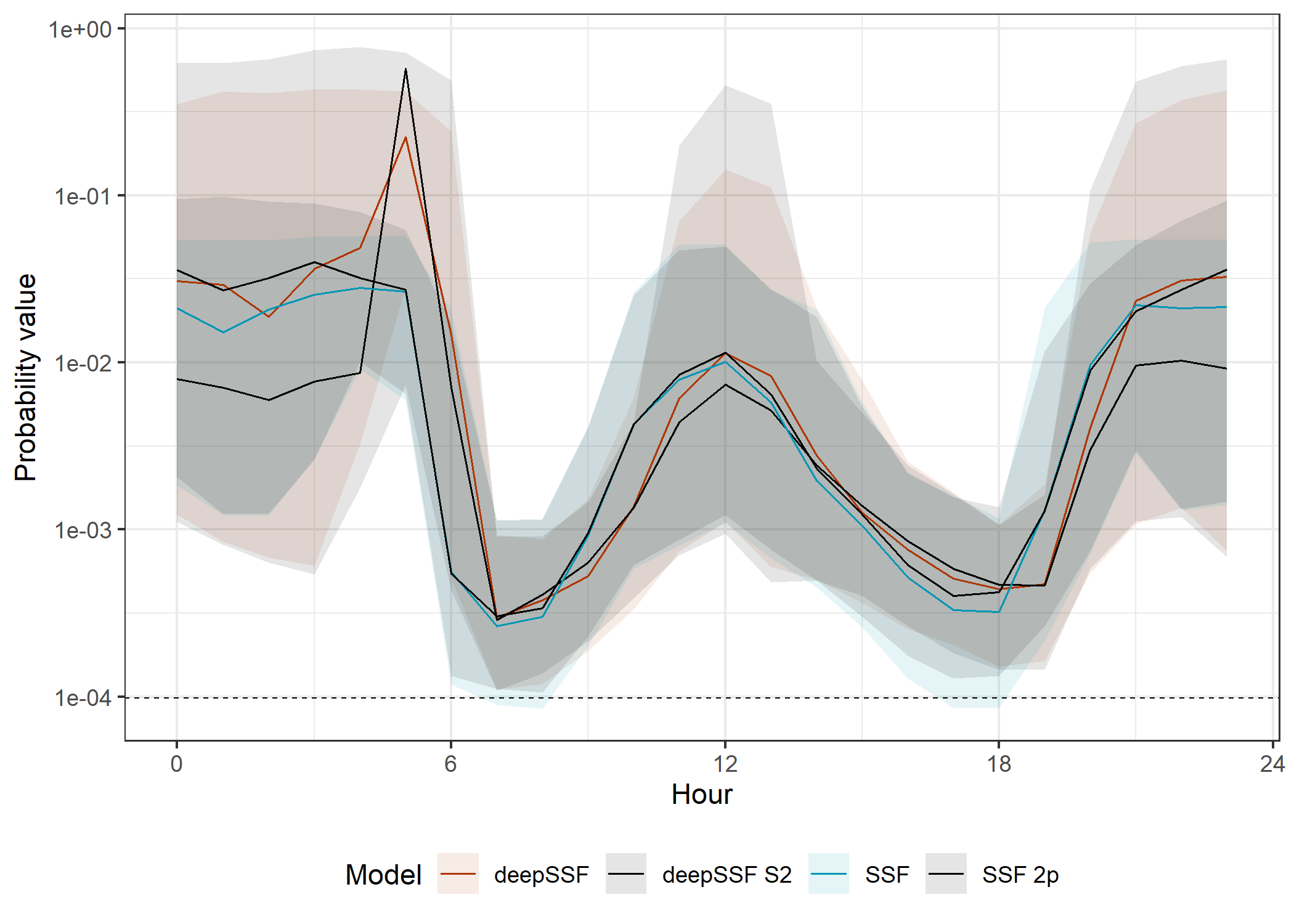
The movement probabilities are much lower during the high movement periods. This is because there are many more cells that the buffalo are likely to move to, and so the probability of moving to any one cell is lower, and the model must spread the prediction probability across many more cells.
The SSF probabilities are also much much lower than the deepSSF probabilities, as explained for the movement probabilities across the tracking period.
deepSSF models
Code
ggplot() +

  # dashed lines containing the SSF probabilities
  # geom_hline(yintercept = 0, alpha = 0.25, linetype = "dashed", linewidth = 0.25) +
  # geom_hline(yintercept = 1.25e-2, alpha = 0.25, linetype = "dashed", linewidth = 0.25) +

  # in sample 50% ribbon
  geom_ribbon(data = validation_all_quantiles_hourly %>%
                filter(probability == "move",
                       id == focal_id,
                       grepl("deepSSF", model)),
              aes(x = hour_t1,
                  ymin = q25,
                  ymax = q75,
                  fill = model,
                  group = interaction(id, model)),
              alpha = ribbon_50_alpha) +

  # in sample mean line
  geom_line(data = validation_all_quantiles_hourly %>%
              filter(probability == "move",
                     id == focal_id,
                     grepl("deepSSF", model)),
            aes(x = hour_t1,
                y = average_prob,
                colour = model,
                group = interaction(id, model)),
            linewidth = primary_linewidth) +

  # dashed line for uniform probability
  geom_hline(yintercept = uniform_prob, linetype = "dashed", linewidth = 0.25) +

  scale_fill_manual(name = "Model",
                     values = c("#E25834", "#000000"),
                    labels = c("deepSSF", "deepSSF S2")) +

  scale_color_manual(name = "Model",
                     values = c("#E25834", "#000000"),
                    labels = c("deepSSF", "deepSSF S2")) +

  scale_y_continuous("Probability value") +
  scale_x_continuous("Hour", seq(0,24,6)) +
  theme_bw() +
  theme(legend.position = "bottom")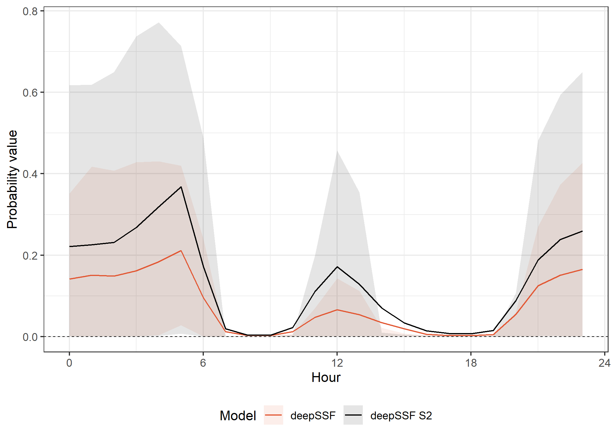
SSF models
Code
ggplot() +

  # in sample 50% ribbon
  geom_ribbon(data = validation_all_quantiles_hourly %>%
                filter(probability == "move",
                       id == focal_id,
                       !grepl("deepSSF", model)),
              aes(x = hour_t1,
                  ymin = q25,
                  ymax = q75,
                  fill = model,
                  group = interaction(id, model)),
              alpha = ribbon_50_alpha) +

  # in sample mean line
  geom_line(data = validation_all_quantiles_hourly %>%
              filter(probability == "move",
                     id == focal_id,
                     !grepl("deepSSF", model)),
            aes(x = hour_t1,
                y = average_prob,
                colour = model,
                group = interaction(id, model)),
            linewidth = primary_linewidth) +

  # dashed line for uniform probability
  geom_hline(yintercept = uniform_prob, linetype = "dashed", linewidth = 0.25) +

  scale_fill_manual(name = "Model",
                     values = c("#0096B5", "#26185F"),
                    labels = c("SSF", "SSF 2p")) +

  scale_color_manual(name = "Model",
                     values = c("#0096B5", "#26185F"),
                    labels = c("SSF", "SSF 2p")) +

    scale_y_continuous("Probability value",
                     position = "right") +

  scale_x_continuous("Hour", seq(0,24,6)) +
  # coord_cartesian(ylim = c(0, 1.25e-2)) +
  theme_bw() +
  theme(legend.position = "bottom")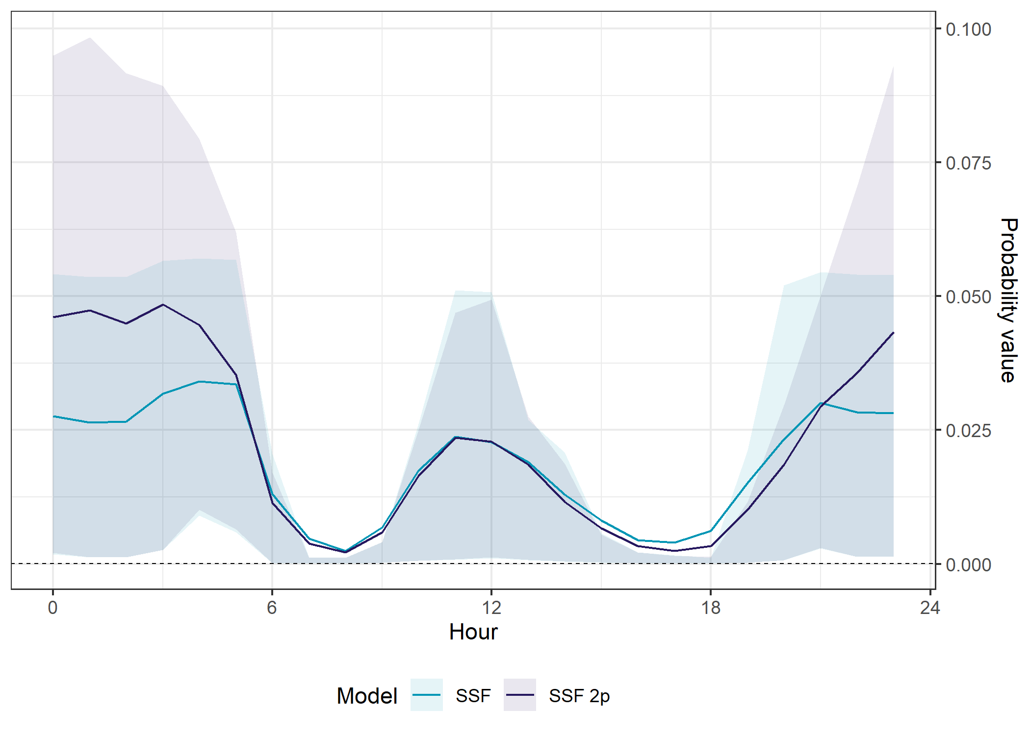
The SSF models perform similarly, expect at night, where the temporally dynamic performs much better in- and out-of-sample.
Next-step probability across the day
All models
Code
ggplot() +

  # dashed lines containing the SSF probabilities
  # geom_hline(yintercept = 0, alpha = 0.25, linetype = "dashed", linewidth = 0.25) +
  # geom_hline(yintercept = 3e-4, alpha = 0.25, linetype = "dashed", linewidth = 0.25) +

  # in sample 50% ribbon
  geom_ribbon(data = validation_all_quantiles_hourly %>%
                filter(probability == "next_step",
                       id == focal_id),
              aes(x = hour_t1,
                  ymin = q25,
                  ymax = q75,
                  fill = model,
                  group = interaction(id, model)),
              alpha = ribbon_50_alpha) +

  # in sample mean line
  geom_line(data = validation_all_quantiles_hourly %>%
              filter(probability == "next_step",
                     id == focal_id),
            aes(x = hour_t1,
                y = average_prob,
                colour = model,
                group = interaction(id, model)),
            linewidth = 0.35) +

  # dashed line for uniform probability
  geom_hline(yintercept = uniform_prob, linetype = "dashed", linewidth = 0.25) +

  scale_fill_manual(name = "Model",
                     values = c("#AF3602", "#000000", "#0096B5", "#000000"),
                    labels = c("deepSSF", "deepSSF S2", "SSF", "SSF 2p")) +

  scale_color_manual(name = "Model",
                     values = c("#AF3602", "#000000", "#0096B5", "#000000"),
                    labels = c("deepSSF", "deepSSF S2", "SSF", "SSF 2p")) +

  # scale_y_continuous("Probability value") +
  scale_y_log10("Probability value") +
  scale_x_continuous("Hour", breaks = seq(0,24,6)) +
  theme_bw() +
  theme(legend.position = "bottom")
Median
Code
ggplot() +

  # dashed lines containing the SSF probabilities
  # geom_hline(yintercept = 0, alpha = 0.25, linetype = "dashed", linewidth = 0.25) +
  # geom_hline(yintercept = 3e-4, alpha = 0.25, linetype = "dashed", linewidth = 0.25) +

  # in sample 50% ribbon
  geom_ribbon(data = validation_all_quantiles_hourly %>%
                filter(probability == "next_step",
                       id == focal_id),
              aes(x = hour_t1,
                  ymin = q25,
                  ymax = q75,
                  fill = model,
                  group = interaction(id, model)),
              alpha = ribbon_50_alpha) +

  # in sample mean line
  geom_line(data = validation_all_quantiles_hourly %>%
              filter(probability == "next_step",
                     id == focal_id),
            aes(x = hour_t1,
                y = q50,
                colour = model,
                group = interaction(id, model)),
            linewidth = 0.35) +

  # dashed line for uniform probability
  geom_hline(yintercept = uniform_prob, linetype = "dashed", linewidth = 0.25) +

  scale_fill_manual(name = "Model",
                     values = c("#AF3602", "#000000", "#0096B5", "#000000"),
                    labels = c("deepSSF", "deepSSF S2", "SSF", "SSF 2p")) +

  scale_color_manual(name = "Model",
                     values = c("#AF3602", "#000000", "#0096B5", "#000000"),
                    labels = c("deepSSF", "deepSSF S2", "SSF", "SSF 2p")) +

  # scale_y_continuous("Probability value") +
  scale_y_log10("Probability value") +
  scale_x_continuous("Hour", breaks = seq(0,24,6)) +
  theme_bw() +
  theme(legend.position = "bottom")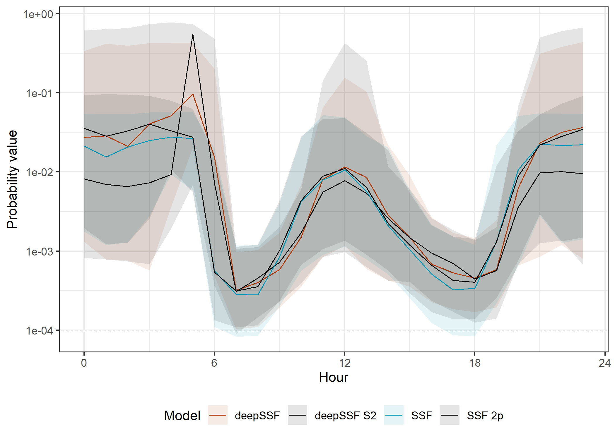
deepSSF models
Code
ggplot() +

  # dashed lines containing the SSF probabilities
  # geom_hline(yintercept = 0, alpha = 0.25, linetype = "dashed", linewidth = 0.25) +
  # geom_hline(yintercept = 1.25e-2, alpha = 0.25, linetype = "dashed", linewidth = 0.25) +

  # in sample 50% ribbon
  geom_ribbon(data = validation_all_quantiles_hourly %>%
                filter(probability == "next_step",
                       id == focal_id,
                       grepl("deepSSF", model)),
              aes(x = hour_t1,
                  ymin = q25,
                  ymax = q75,
                  fill = model,
                  group = interaction(id, model)),
              alpha = ribbon_50_alpha) +

  # in sample mean line
  geom_line(data = validation_all_quantiles_hourly %>%
              filter(probability == "next_step",
                     id == focal_id,
                     grepl("deepSSF", model)),
            aes(x = hour_t1,
                y = average_prob,
                colour = model,
                group = interaction(id, model)),
            linewidth = primary_linewidth) +

  # dashed line for uniform probability
  geom_hline(yintercept = uniform_prob, linetype = "dashed", linewidth = 0.25) +

  scale_fill_manual(name = "Model",
                     values = c("#E25834", "#000000"),
                    labels = c("deepSSF", "deepSSF S2")) +

  scale_color_manual(name = "Model",
                     values = c("#E25834", "#000000"),
                    labels = c("deepSSF", "deepSSF S2")) +

  scale_y_continuous("Probability value") +
  scale_x_continuous("Hour", seq(0,24,6)) +
  theme_bw() +
  theme(legend.position = "bottom")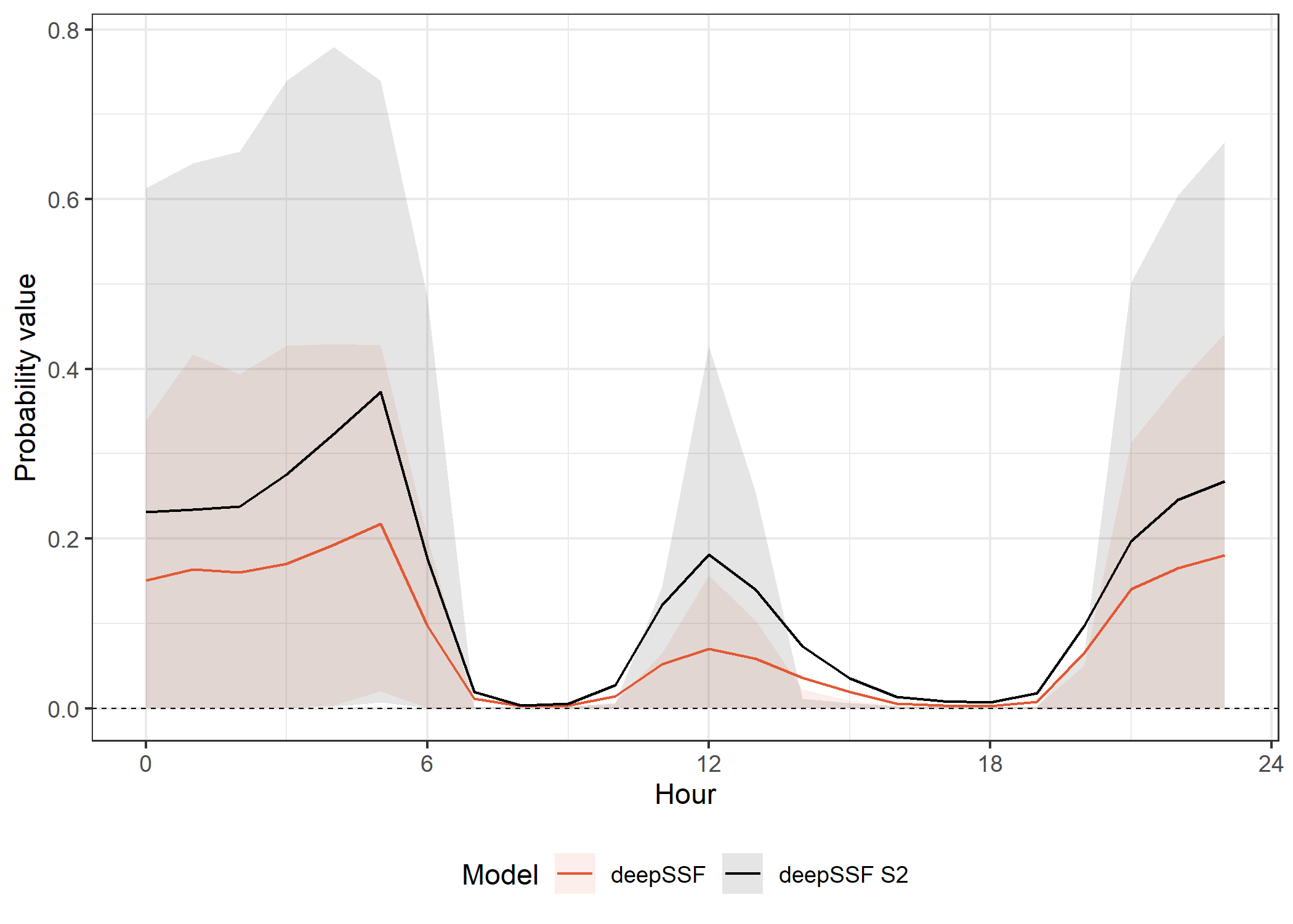
SSF models
Code
ggplot() +

  # in sample 50% ribbon
  geom_ribbon(data = validation_all_quantiles_hourly %>%
                filter(probability == "next_step",
                       id == focal_id,
                       !grepl("deepSSF", model)),
              aes(x = hour_t1,
                  ymin = q25,
                  ymax = q75,
                  fill = model,
                  group = interaction(id, model)),
              alpha = ribbon_50_alpha) +

  # in sample mean line
  geom_line(data = validation_all_quantiles_hourly %>%
              filter(probability == "next_step",
                     id == focal_id,
                     !grepl("deepSSF", model)),
            aes(x = hour_t1,
                y = average_prob,
                colour = model,
                group = interaction(id, model)),
            linewidth = primary_linewidth) +

  # dashed line for uniform probability
  geom_hline(yintercept = uniform_prob, linetype = "dashed", linewidth = 0.25) +

  scale_fill_manual(name = "Model",
                     values = c("#0096B5", "#26185F"),
                    labels = c("SSF", "SSF 2p")) +

  scale_color_manual(name = "Model",
                     values = c("#0096B5", "#26185F"),
                    labels = c("SSF", "SSF 2p")) +

    scale_y_continuous("Probability value",
                     position = "right") +

  scale_x_continuous("Hour", seq(0,24,6)) +
  # coord_cartesian(ylim = c(0, 1.25e-2)) +
  theme_bw() +
  theme(legend.position = "bottom")