for j in range(0, len(csv_files)):
# Read one of the CSV files into a DataFrame
buffalo_df = pd.read_csv(csv_files[j])
# Extract ID from the string for saving the file
buffalo_id = csv_files[j][55:59]
# Lag the bearing values in column 'A' by one index (to get the previous bearing)
buffalo_df['bearing_tm1'] = buffalo_df['bearing'].shift(1)
# Pad the missing value with a specified value, e.g., 0
buffalo_df['bearing_tm1'] = buffalo_df['bearing_tm1'].fillna(0)
test_data = buffalo_df
n_samples = len(test_data)
# create empty vectors to store the predicted probabilities
habitat_probs = np.repeat(0., n_samples)
move_probs = np.repeat(0., n_samples)
next_step_probs = np.repeat(0., n_samples)
# start at 1 so the bearing at t - 1 is available
for i in range(1, n_samples):
sample = test_data.iloc[i]
# Current location (x1, y1)
x = sample['x1_']
y = sample['y1_']
# Convert geographic coordinates to pixel coordinates
px, py = ~raster_transform * (x, y)
# Next step location (x2, y2)
x2 = sample['x2_']
y2 = sample['y2_']
# Convert geographic coordinates to pixel coordinates
px2, py2 = ~raster_transform * (x2, y2)
# The difference in x and y coordinates
d_x = x2 - x
d_y = y2 - y
# print('d_x and d_y are ', d_x, d_y) # Debugging
# Temporal covariates
hour_t2_sin = sample['hour_t2_sin']
hour_t2_cos = sample['hour_t2_cos']
yday_t2_sin = sample['yday_t2_sin']
yday_t2_cos = sample['yday_t2_cos']
# Bearing of previous step (t - 1)
bearing = sample['bearing_tm1']
# Day of the year
yday = sample['yday_t2']
# Convert day of the year to month index
month_index = day_to_month_index(yday)
# print(month_index)
# Adjust month_index to range from 1 to 12
month_index = (month_index - 1) % 12 + 1
# for sentinel 2 data
selected_month = f'2019_{month_index:02d}'
# Get the normalized data for the selected month
s2_data = data_dict[selected_month]
# Convert the NumPy array to a PyTorch tensor
s2_tensor = torch.from_numpy(s2_data)
s2_tensor = s2_tensor.float() # Ensure the tensor is of type float
# print(s2_tensor.shape)
# Get the subset of the Sentinel-2 bands
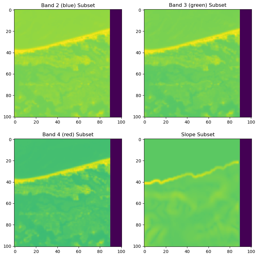
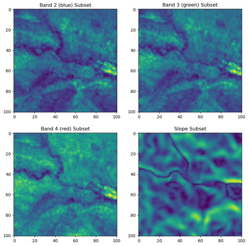
s2_b1_subset, origin_x, origin_y = subset_function(s2_tensor[0,:,:], x, y, window_size, raster_transform)
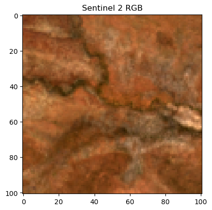
s2_b2_subset, origin_x, origin_y = subset_function(s2_tensor[1,:,:], x, y, window_size, raster_transform)
s2_b3_subset, origin_x, origin_y = subset_function(s2_tensor[2,:,:], x, y, window_size, raster_transform)
s2_b4_subset, origin_x, origin_y = subset_function(s2_tensor[3,:,:], x, y, window_size, raster_transform)
s2_b5_subset, origin_x, origin_y = subset_function(s2_tensor[4,:,:], x, y, window_size, raster_transform)
s2_b6_subset, origin_x, origin_y = subset_function(s2_tensor[5,:,:], x, y, window_size, raster_transform)
s2_b7_subset, origin_x, origin_y = subset_function(s2_tensor[6,:,:], x, y, window_size, raster_transform)
s2_b8_subset, origin_x, origin_y = subset_function(s2_tensor[7,:,:], x, y, window_size, raster_transform)
s2_b8a_subset, origin_x, origin_y = subset_function(s2_tensor[8,:,:], x, y, window_size, raster_transform)
s2_b9_subset, origin_x, origin_y = subset_function(s2_tensor[9,:,:], x, y, window_size, raster_transform)
s2_b11_subset, origin_x, origin_y = subset_function(s2_tensor[10,:,:], x, y, window_size, raster_transform)
s2_b12_subset, origin_x, origin_y = subset_function(s2_tensor[11,:,:], x, y, window_size, raster_transform)
# Get the subset of the slope landscape
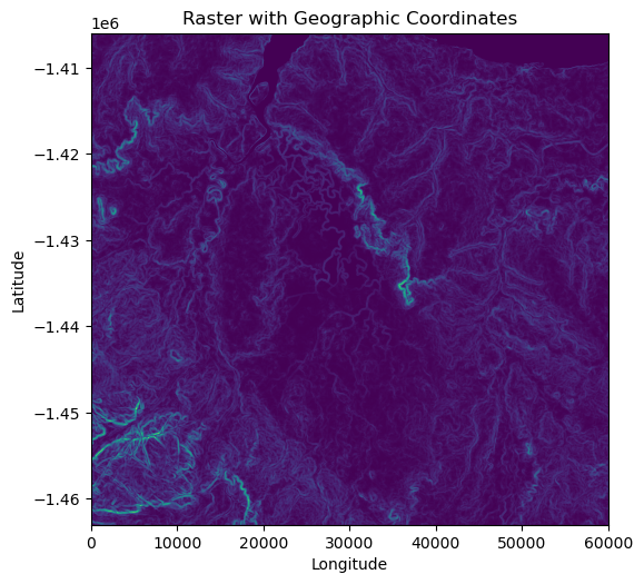
slope_subset, origin_x, origin_y = subset_function(slope_landscape_norm, x, y, window_size, raster_transform)
# Stack the channels along a new axis; here, 1 is commonly used for channel axis in PyTorch
x1 = torch.stack([s2_b1_subset,
s2_b2_subset,
s2_b3_subset,
s2_b4_subset,
s2_b5_subset,
s2_b6_subset,
s2_b7_subset,
s2_b8_subset,
s2_b8a_subset,
s2_b9_subset,
s2_b11_subset,
s2_b12_subset,
slope_subset], dim=0)
x1 = x1.unsqueeze(0)
# print(x1.shape)
# print('origin_x and origin_y are ', origin_x, origin_y)
px2_subset = px2 - origin_x
py2_subset = py2 - origin_y
# print('delta origin_x and origin_y are ', px2_subset, py2_subset)
# print('delta origin_x and origin_y are ', int(px2_subset), int(py2_subset))
# Convert lists to PyTorch tensors
hour_t2_sin_tensor = torch.tensor(hour_t2_sin).float()
hour_t2_cos_tensor = torch.tensor(hour_t2_cos).float()
yday_t2_sin_tensor = torch.tensor(yday_t2_sin).float()
yday_t2_cos_tensor = torch.tensor(yday_t2_cos).float()
# Stack tensors column-wise
x2 = torch.stack((hour_t2_sin_tensor.unsqueeze(0),
hour_t2_cos_tensor.unsqueeze(0),
yday_t2_sin_tensor.unsqueeze(0),
yday_t2_cos_tensor.unsqueeze(0)),
dim=1)
# print(x2)
# print(x2.shape)
# put bearing in the correct dimension (batch_size, 1)
bearing = torch.tensor(bearing).float().unsqueeze(0).unsqueeze(0)
# print(bearing)
# print(bearing.shape)
# -------------------------------------------------------------------------
# Run the model
# -------------------------------------------------------------------------
model_output = model((x1, x2, bearing))
# -------------------------------------------------------------------------
# Habitat selection probability
# -------------------------------------------------------------------------
hab_density = model_output.detach().cpu().numpy()[0,:,:,0]
hab_density_exp = np.exp(hab_density)
# print(np.sum(hab_density_exp)) # Should be 1
# Store the probability of habitat selection at the location of x2, y2
# These probabilities are normalised in the model function
habitat_probs[i] = hab_density_exp[(int(py2_subset), int(px2_subset))]
# print('Habitat probability value = ', habitat_probs[i])
# -------------------------------------------------------------------------
# Movement probability
# -------------------------------------------------------------------------
move_density = model_output.detach().cpu().numpy()[0,:,:,1]
move_density_exp = np.exp(move_density)
# print(np.sum(move_density_exp)) # Should be 1
# Store the movement probability at the location of x2, y2
# These probabilities are normalised in the model function
move_probs[i] = move_density_exp[(int(py2_subset), int(px2_subset))]
# print('Movement probability value = ', move_probs[i])
# -------------------------------------------------------------------------
# Next step probability
# -------------------------------------------------------------------------
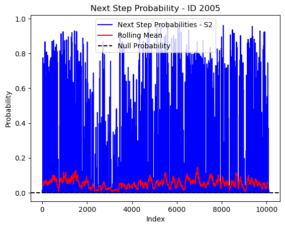
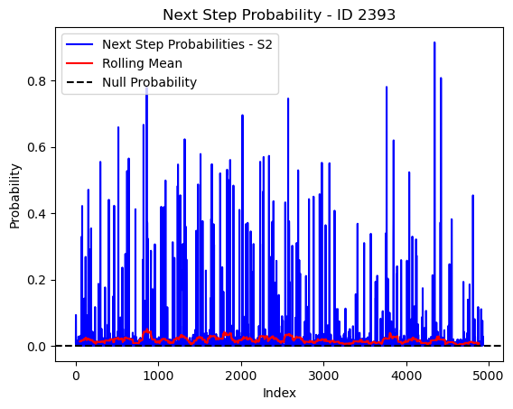
step_density = hab_density + move_density
step_density_exp = np.exp(step_density)
# print('Sum of step density exp = ', np.sum(step_density_exp)) # Won't be 1
step_density_exp_norm = step_density_exp / np.sum(step_density_exp)
# print('Sum of step density exp norm = ', np.sum(step_density_exp_norm)) # Should be 1
# Extract the value of the covariates at the location of x2, y2
next_step_probs[i] = step_density_exp_norm[(int(py2_subset), int(px2_subset))]
# print('Next-step probability value = ', next_step_probs[i])
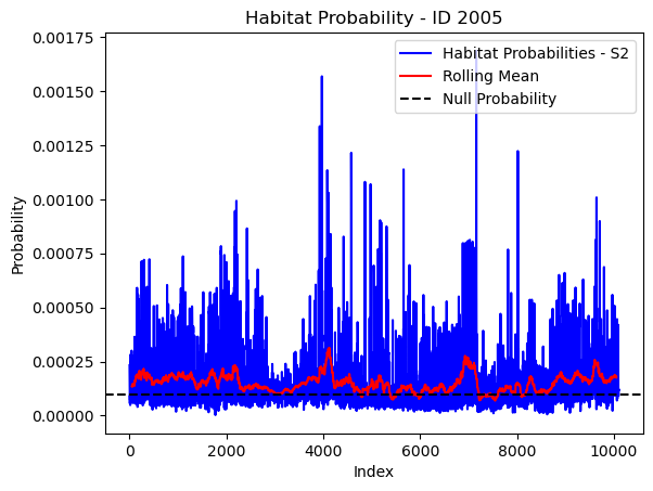
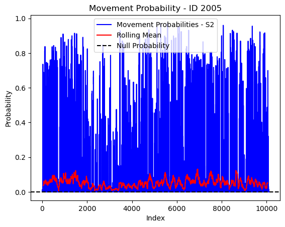
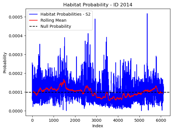
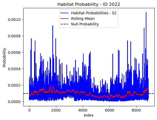
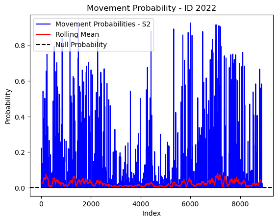
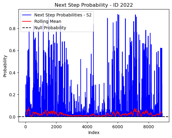
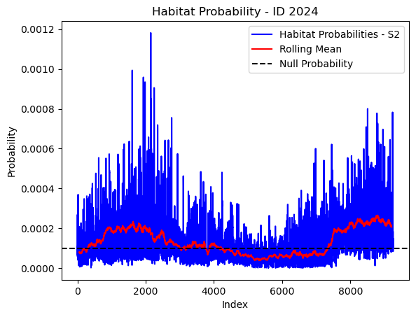
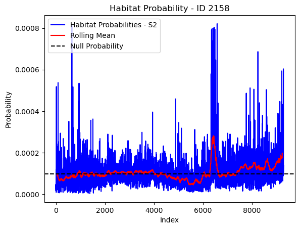
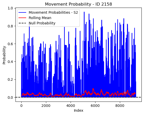
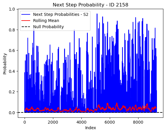
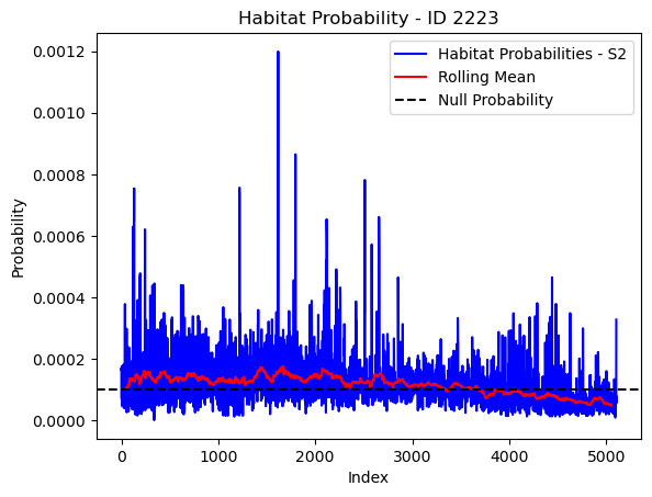
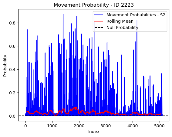
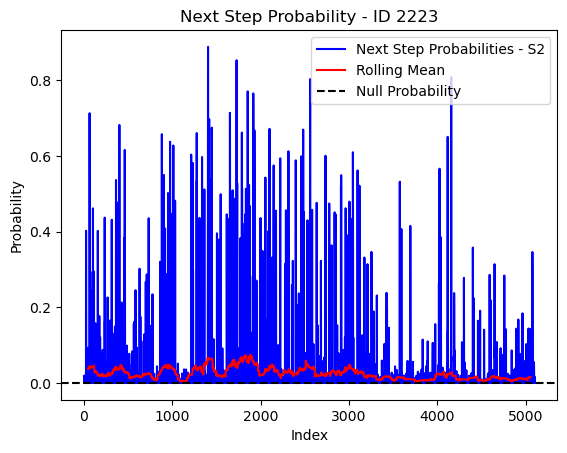
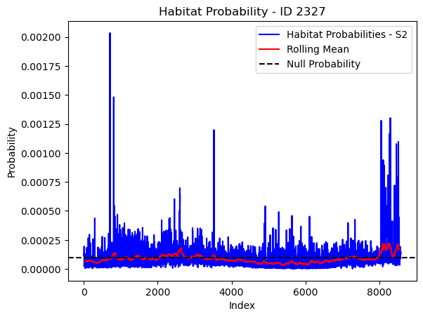
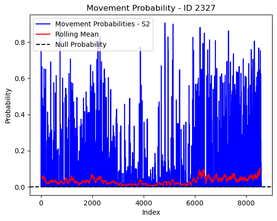
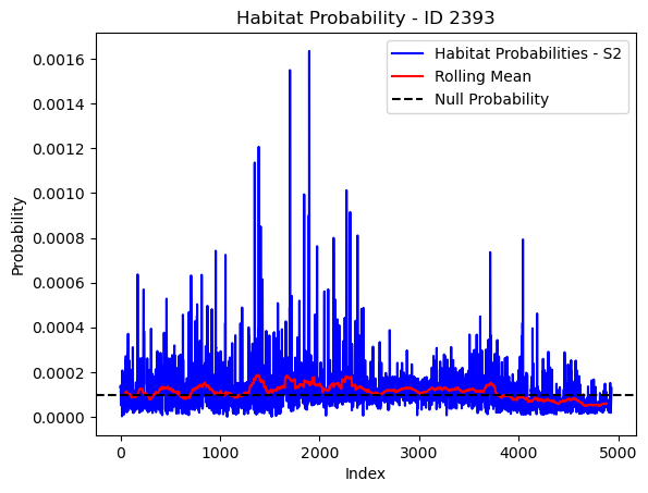
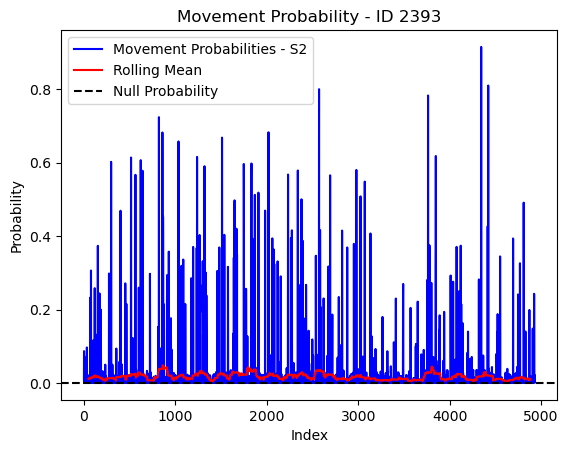
# Convert to pandas Series and compute rolling mean
rolling_mean_habitat = pd.Series(habitat_probs).rolling(window=window_size, center=True).mean()
rolling_mean_movement = pd.Series(move_probs).rolling(window=window_size, center=True).mean()
rolling_mean_next_step = pd.Series(next_step_probs).rolling(window=window_size, center=True).mean()
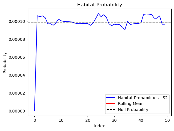
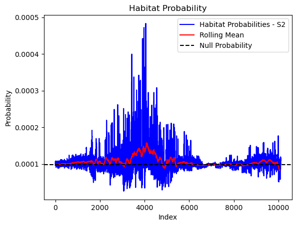
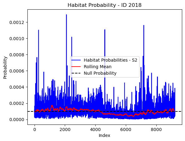
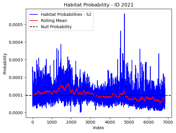
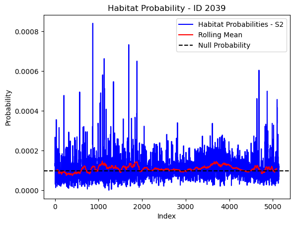
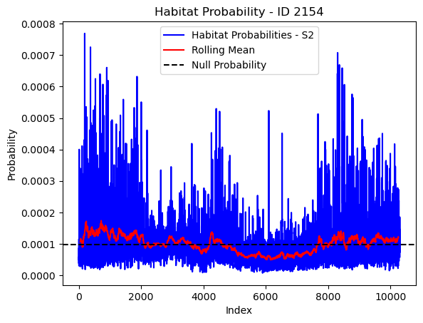
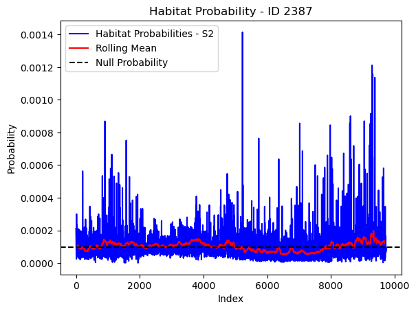
# Plot the habitat probs through time as a line graph
plt.plot(habitat_probs[habitat_probs > 0], color='blue', label='Habitat Probabilities - S2')
plt.plot(rolling_mean_habitat[rolling_mean_habitat > 0], color='red', label='Rolling Mean')
plt.axhline(y=null_prob, color='black', linestyle='--', label='Null Probability') # null probs
plt.xlabel('Index')
plt.ylabel('Probability')
plt.title(f'Habitat Probability - ID {buffalo_id}')
plt.legend() # Add legend to differentiate lines
plt.show()
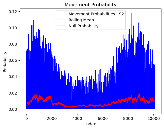
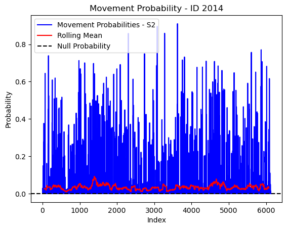
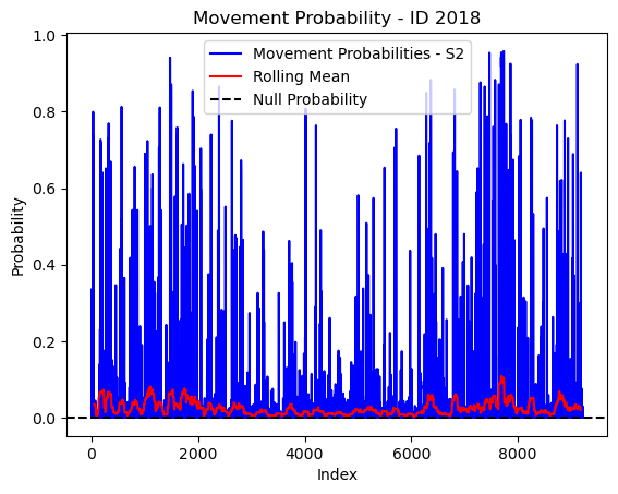
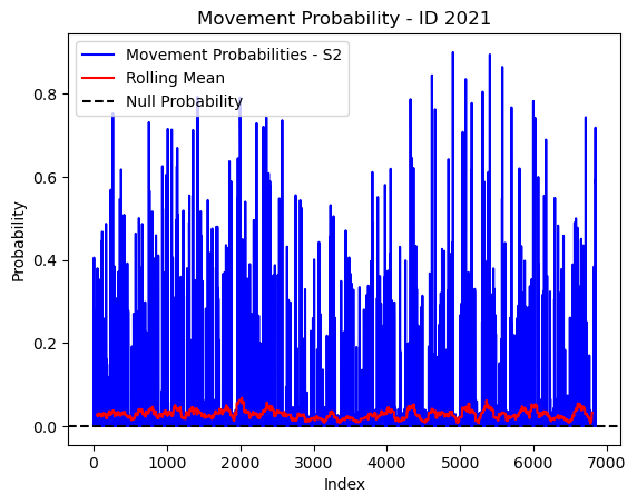
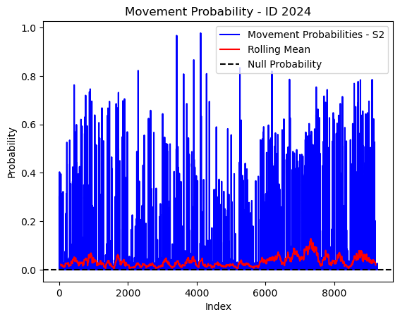
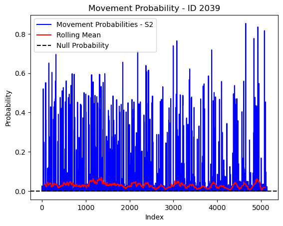
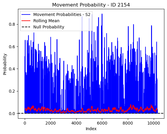
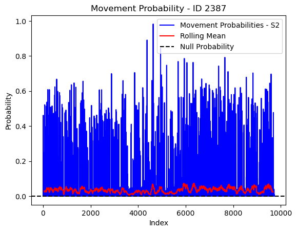
# Plot the movement probs through time as a line graph
plt.plot(move_probs[move_probs > 0], color='blue', label='Movement Probabilities - S2')
plt.plot(rolling_mean_movement[rolling_mean_movement > 0], color='red', label='Rolling Mean')
plt.axhline(y=null_prob, color='black', linestyle='--', label='Null Probability') # null probs
plt.xlabel('Index')
plt.ylabel('Probability')
plt.title(f'Movement Probability - ID {buffalo_id}')
plt.legend() # Add legend to differentiate lines
plt.show()
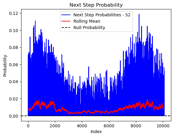
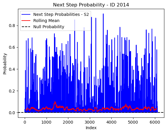
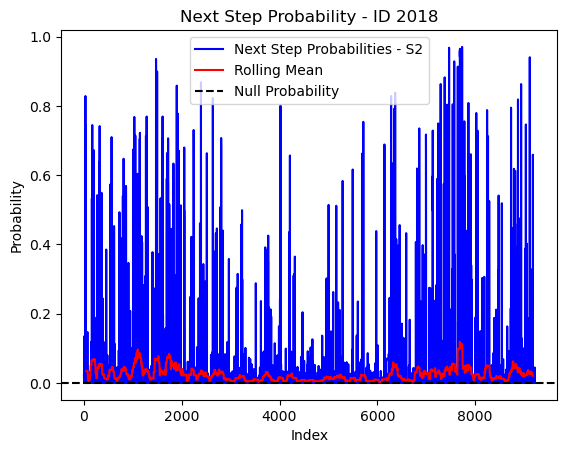
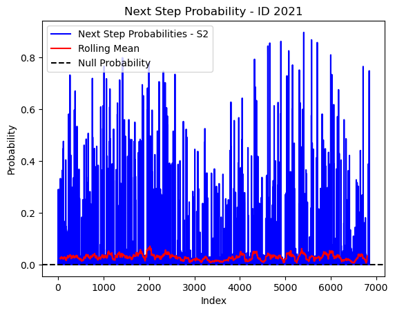
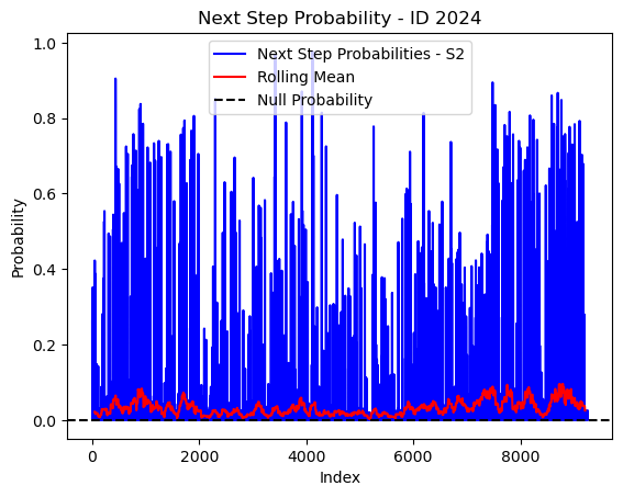
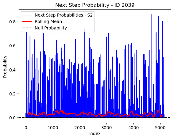
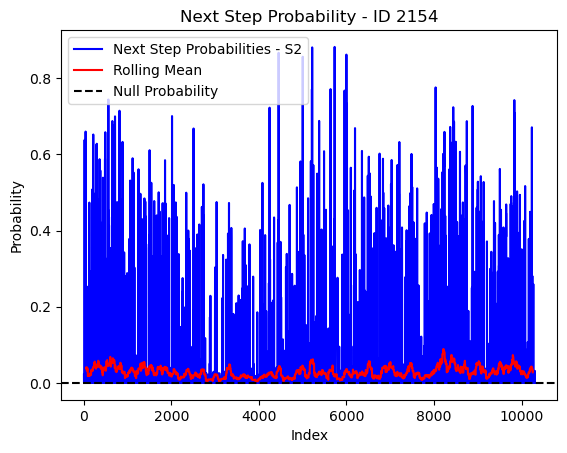
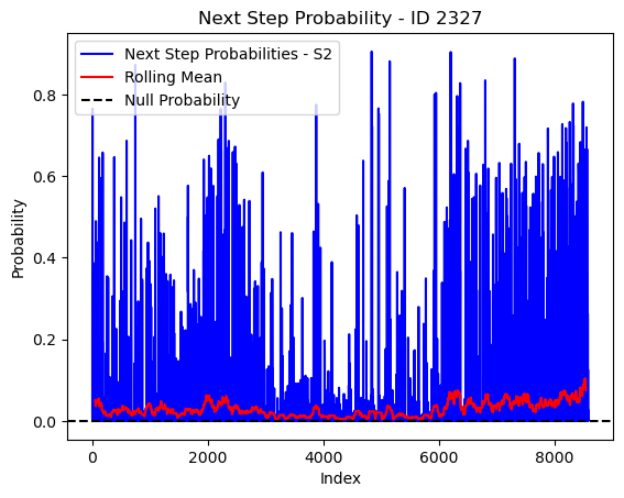
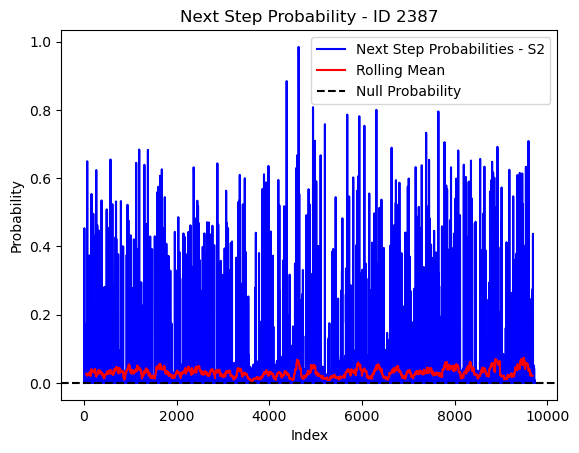
# Plot the next step probs through time as a line graph
plt.plot(next_step_probs[next_step_probs > 0], color='blue', label='Next Step Probabilities - S2')
plt.plot(rolling_mean_next_step[rolling_mean_next_step > 0], color='red', label='Rolling Mean')
plt.axhline(y=null_prob, color='black', linestyle='--', label='Null Probability') # null probs
plt.xlabel('Index')
plt.ylabel('Probability')
plt.title(f'Next Step Probability - ID {buffalo_id}')
plt.legend() # Add legend to differentiate lines
plt.show()
# Save the data to a CSV file
csv_filename = f'{output_dir}/deepSSF_id{buffalo_id}_n{len(test_data)}_{today_date}.csv'
print(f'File saved as: {csv_filename}')
buffalo_df.to_csv(csv_filename, index=True)