SSF Validation

Similar to the deepSSF next-step validation scripts, we can validate the fitted SSF models by assessing the predicted probability values at the location of the next step. We can do this for the movement, habitat selection and next-step probability surfcaes, providing information about the accuracy of each of these processes, and how that changes through time.
We fitted the SSF models (with and without temporal dynamics) in the SSF Model Fitting script, and we can use the fitted parameters to generate the movement, habitat sele
Whilst the realism and emergent properties of simulated trajectories are difficult to assess, we can validate the deepSSF models on their predictive performance at the next step, for each of the habitat selection, movement and next-step probability surfaces. Ensuring that the probability surfaces are normalised to sum to one, they can be compared to the predictions of typical step selection functions when the same probability surfaces are generated for the same local covariates. This approach not only allows for comparison between models, but can be informative as to when in the observed trajectory the model performs well or poorly, which can be analysed across the entire tracking period or for each hour of the day, and can lead to critical evaluation of the covariates that are used by the models and allow for model refinement.
Loading packages
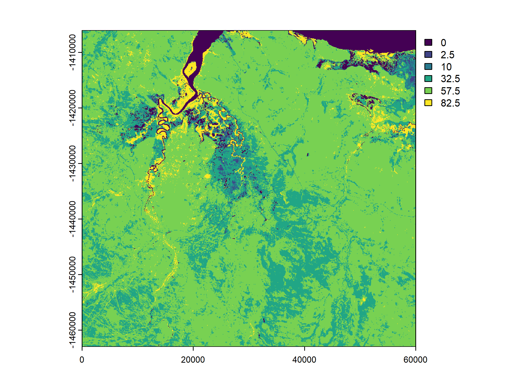
Reading in the environmental covariates
Code
ndvi_projected <- rast("mapping/cropped rasters/ndvi_GEE_projected_watermask20230207.tif")
terra::time(ndvi_projected) <- as.POSIXct(lubridate::ymd("2018-01-01") + months(0:23))
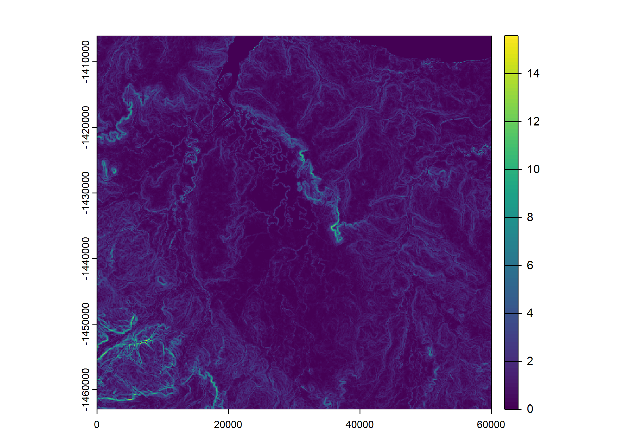
slope <- rast("mapping/cropped rasters/slope_raster.tif")
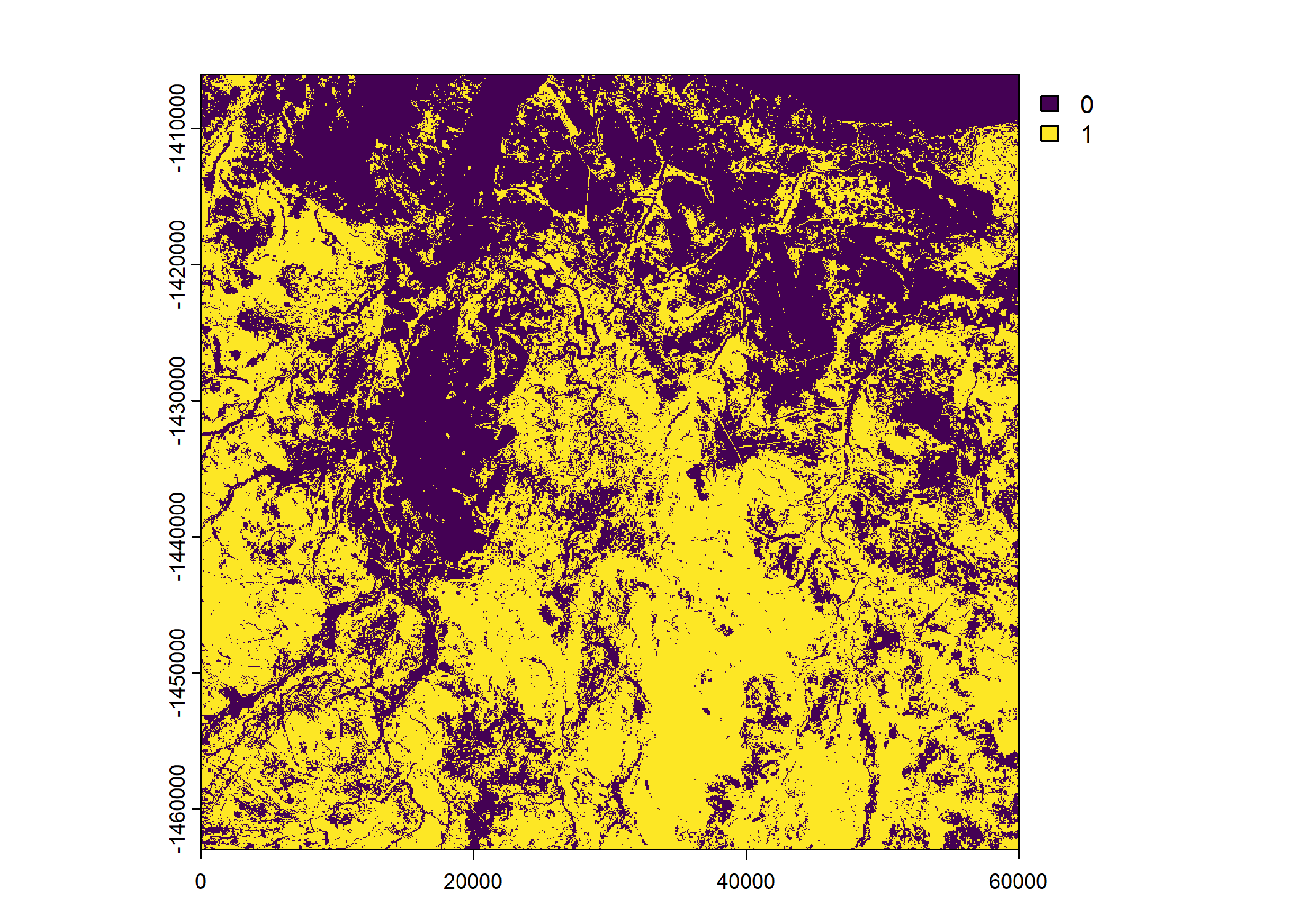
veg_herby <- rast("mapping/cropped rasters/veg_herby.tif")
canopy_cover <- rast("mapping/cropped rasters/canopy_cover.tif")
# change the names (these will become the column names when extracting
# covariate values at the used and random steps)
names(ndvi_projected) <- rep("ndvi", terra::nlyr(ndvi_projected))
names(slope) <- "slope"
names(veg_herby) <- "veg_herby"
names(canopy_cover) <- "canopy_cover"
# to plot the rasters
plot(ndvi_projected)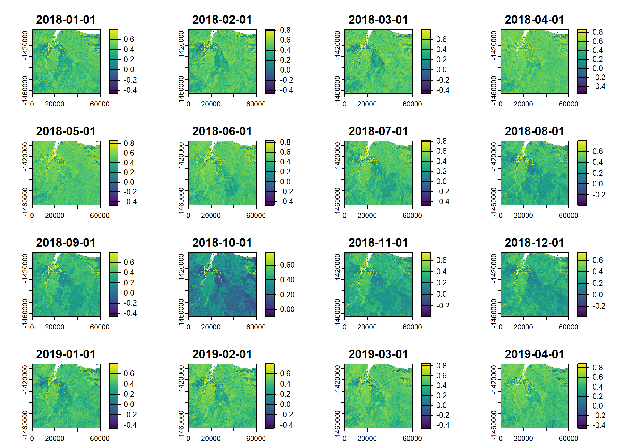
Generating the data to fit a deepSSF model
Set up the spatial extent of the local covariates
Code
# get the resolution from the covariates
res <- terra::res(ndvi_projected)[1]

# how much to trim on either side of the location,
# this will determine the extent of the spatial inputs to the deepSSF model
buffer <- 1250 + (res/2)
# calculate the number of cells in each axis
nxn_cells <- buffer*2/res

# hourly lag - to set larger time differences between locations
hourly_lag <- 1
Evaluate next-step ahead predictions
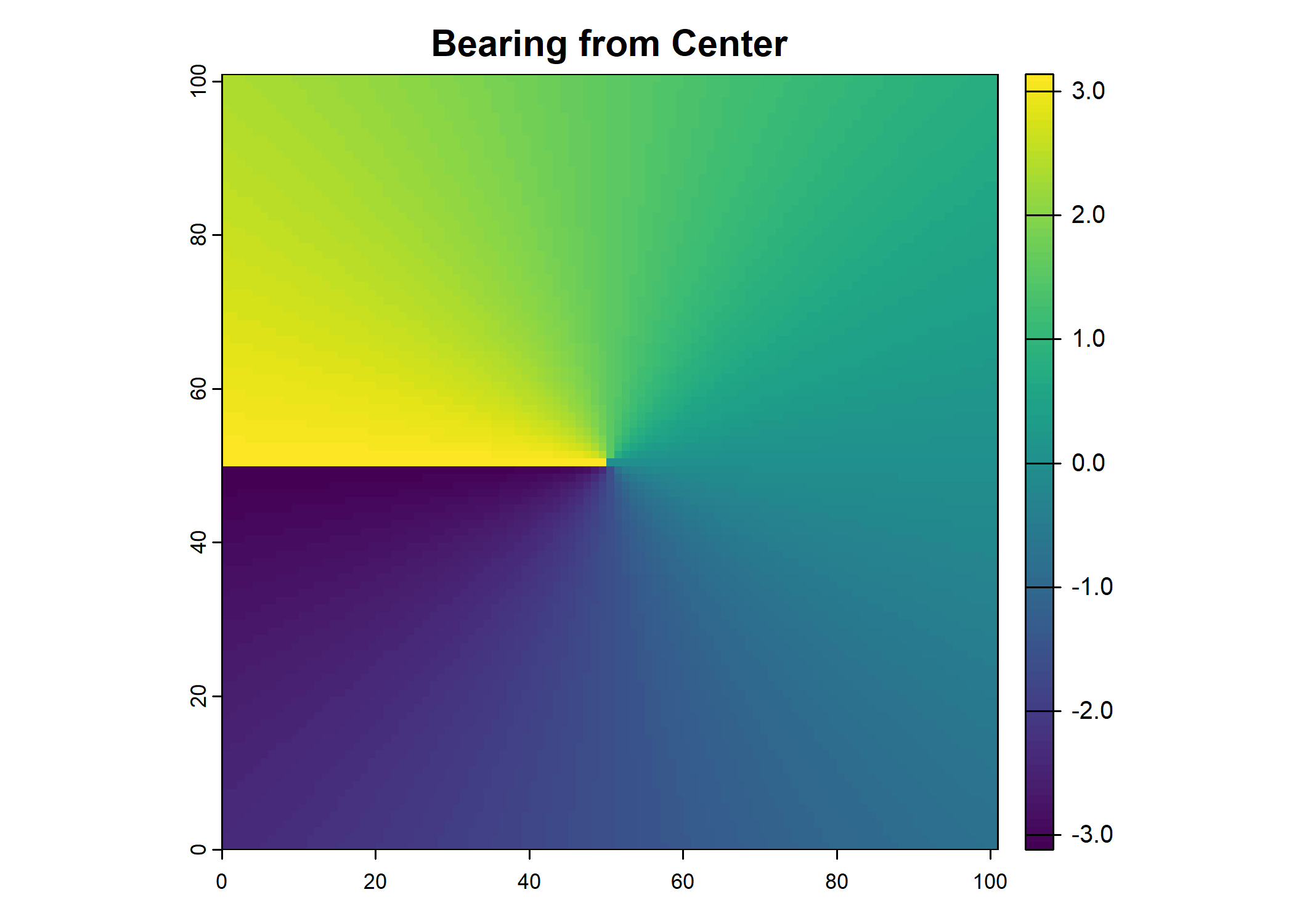
Create distance and bearing layers for the movement probability
Code
image_dim <- 101
pixel_size <- 25
center <- image_dim %/% 2

# Create matrices of indices
x <- matrix(rep(0:(image_dim - 1), image_dim), nrow = image_dim, byrow = TRUE)
y <- matrix(rep(0:(image_dim - 1), each = image_dim), nrow = image_dim, byrow = TRUE)

# Compute the distance layer
distance_layer <- sqrt((pixel_size * (x - center))^2 + (pixel_size * (y - center))^2)

# Change the center cell to the average distance from the center to the edge of the pixel
distance_layer[center + 1, center + 1] <- 0.56 * pixel_size

# Compute the bearing layer
bearing_layer <- atan2(center - y, x - center)

# Convert the distance and bearing matrices to raster layers
distance_layer <- rast(distance_layer)
bearing_layer <- rast(bearing_layer)

# Optional: Plot the distance and bearing rasters
plot(distance_layer, main = "Distance from Center")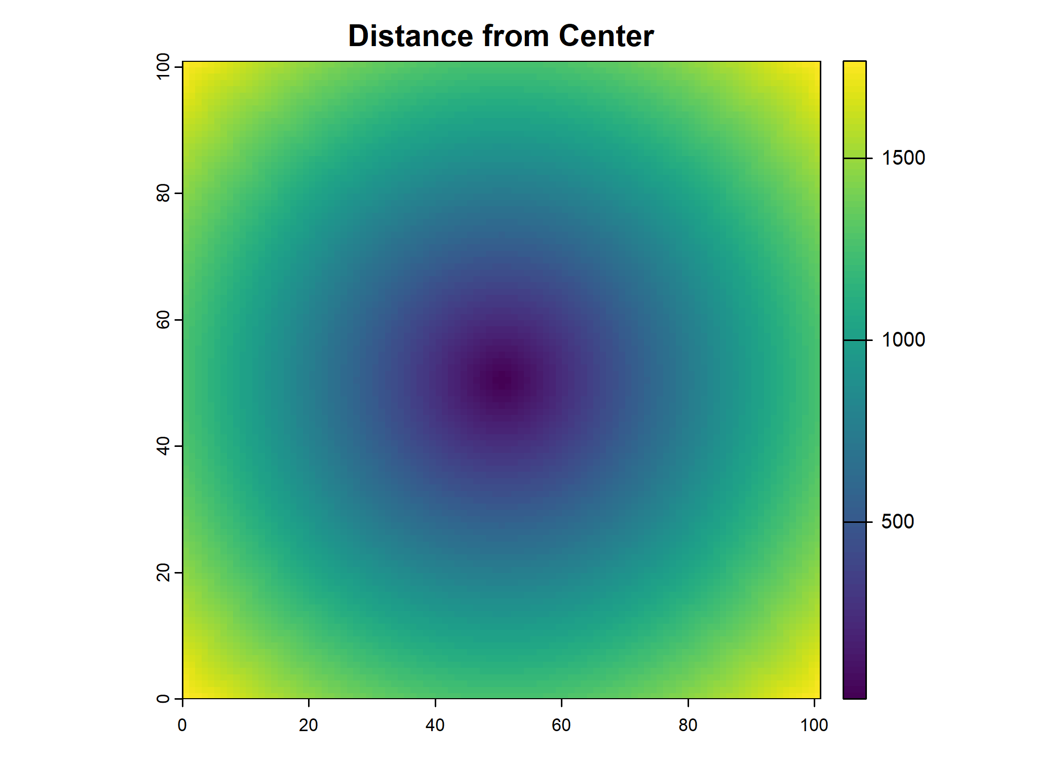
Calculating the habitat selection probabilities
The habitat selection term of a step selection function is typically modelled analogously to a resource-selection function (RSF), that assumes an exponential (log-linear) form as
\[ \omega(\mathbf{X}(s_t); \boldsymbol{\beta}(\tau; \boldsymbol{\alpha})) = \exp(\beta_{1}(\tau; \boldsymbol{\alpha}_1) X_1(s_t) + \cdots + \beta_{n}(\tau; \boldsymbol{\alpha}_n) X_n(s_t)), \]
where \(\boldsymbol{\beta}(\tau; \boldsymbol{\alpha}) = (\beta_{1}(\tau; \boldsymbol{\alpha}_1), \ldots, \beta_{n}(\tau; \boldsymbol{\alpha}_n))\) in our case,
\[ \beta_i(\tau; \boldsymbol{\alpha}_i) = \alpha_{i,0} + \sum_{j = 1}^P \alpha_{i,j} \sin \left(\frac{2j \pi \tau}{T} \right) + \sum_{j = 1}^P \alpha_{i,j + P} \cos \left(\frac{2j \pi \tau}{T} \right), \]
and \(\boldsymbol{\alpha}_i = (\alpha_{i, 0}, \dots, \alpha_{i, 2P})\), where \(P\) is the number of pairs of harmonics, e.g. for \(P = 2\), for each covariate there would be two sine terms and two cosine terms, as well as the linear term denoted by \(\alpha_{i, 0}\). The \(+ P\) term in the \(\alpha\) index of the cosine term ensures that each \(\alpha_i\) coefficient in \(\boldsymbol{\alpha}_i\) is unique.
To aid the computation of the simulations, we can precompute \(\omega(\mathbf{X}(s_t); \boldsymbol{\beta}(\tau; \boldsymbol{\alpha}))\) for each hour prior to running the simulations.
In the dataframe of temporally varying coefficients, for each covariate we have reconstructed \(\beta_{i}(\tau; \boldsymbol{\alpha}_i)\) and discretised for each hour of the day, resulting in \(\beta_{i,\tau}\) for \(i = 1, \ldots, n\) where \(n\) is the number of covariates and \(\tau = 1, \ldots, 24\).
Given these, we can solve \(\omega(\mathbf{X}(s_t); \boldsymbol{\beta}(\tau; \boldsymbol{\alpha}))\) for every hour of the day. This will result in an RSF map for each hour of the day, which we will use in the simulations.
Then, when we do our step selection simulations, we can just subset these maps by the current hour of the day, and extract the values of \(\omega(\mathbf{X}(s_t); \boldsymbol{\beta}(\tau; \boldsymbol{\alpha}))\) for each proposed step location, rather than solving \(\omega(\mathbf{X}(s_t); \boldsymbol{\beta}(\tau; \boldsymbol{\alpha}))\) for every step location.
Calculating the next-step probabilities for the 0p and 2p models
Select model coefficients
Setting up the data
Read in the data of all individuals, which includes the focal or ‘in-sample’ individual that the model was fitted to, as well as the data of the ‘out-of-sample’ individuals that the model has never seen before, and which is from quite a different environmental space (more on the floodplain and closer to the river system).
Code
 [1] "buffalo_2005_data_df_lag_1hr_n10297.csv"
 [2] "buffalo_2014_data_df_lag_1hr_n6572.csv"
 [3] "buffalo_2018_data_df_lag_1hr_n9440.csv"
 [4] "buffalo_2021_data_df_lag_1hr_n6928.csv"
 [5] "buffalo_2022_data_df_lag_1hr_n9099.csv"
 [6] "buffalo_2024_data_df_lag_1hr_n9531.csv"
 [7] "buffalo_2039_data_df_lag_1hr_n5569.csv"
 [8] "buffalo_2154_data_df_lag_1hr_n10417.csv"
 [9] "buffalo_2158_data_df_lag_1hr_n9700.csv"
[10] "buffalo_2223_data_df_lag_1hr_n5310.csv"
[11] "buffalo_2327_data_df_lag_1hr_n8983.csv"
[12] "buffalo_2387_data_df_lag_1hr_n10409.csv"
[13] "buffalo_2393_data_df_lag_1hr_n5299.csv"
[14] "buffalo_temporal_cont_2005_data_df_lag_1hr_n10.csv"
[15] "buffalo_temporal_cont_2005_data_df_lag_1hr_n100.csv"
[16] "buffalo_temporal_cont_2005_data_df_lag_1hr_n10297.csv"
[17] "fixed_buffalo_2005_data_df_lag_1hr_n10297.csv"
Code
ids <- substr(buffalo_data_ids, 9, 12)

# import data
buffalo_id_list <- vector(mode = "list", length = length(buffalo_data_ids))

# read in the data
for(i in 1:length(buffalo_data_ids)){

  buffalo_id_list[[i]] <-  read.csv(paste("buffalo_local_data_id/",
                                             buffalo_data_ids[[i]],
                                             sep = ""))
  buffalo_id_list[[i]]$id <- ids[i]

}
Calculating the next-step probabilities
This scrip takes a long time to run. As we have already calculated the next-step probabilities for all individuals and all steps we will just calculate a subset of the next-step predictions for illustration.
Loop over all individuals and models
This script loops over all individuals and models, and calculates the next-step probabilities for each step of the individual.
Here’s high-level overview of the full chunk below
Outermost loop: for(k in 1:length(buffalo_id_list)) {...}
Data Preparation and Subsetting
- Each buffalo’s trajectory (
data_id) is filtered to retain location steps within the local spatial spatial extent (±1250m). - Any steps with missing data (e.g., turning angle,
ta) are removed. - The data is used to define a local bounding box (
template_raster_crop) for cropping relevant raster datasets. This bounding box covers the extent of all points for that individual, and is for computational efficiency (so the full raster isn’t being subsetted at every step). This is only done once per individual and is not the same as the local cropping done at every step.
- Each buffalo’s trajectory (
Covariate Rasters Cropped to Bounding Box
- NDVI (Normalized Difference Vegetation Index - including squared term)
- Canopy Cover (including squared term)
- Herbaceous Vegetation
- Slope
Middle loop: for(j in 1:length(model_harmonics)) {...}
SSF Models
- The script selects one of the two models:
0p(no temporal harmonics) or2p(temporal harmonics), indicated bymodel_harmonics. - Corresponding coefficients for each model are read from CSV files (e.g.,
"ssf_coefficients/id{focal_id}_{model_harmonics[j]}Daily_coefs_{model_date}.csv"). - Only integer hours are used (filtered via
hour %% 1 == 0).
- The script selects one of the two models:
Inner loop: for (i in 2:n) {..}
Loop Over Steps
For each step in the buffalo’s trajectory:Extract Local Covariates
A subset of each covariate raster is cropped to the step’s spatial extent.Habitat Selection Probability
- Relevant coefficients (e.g.,
ndvi,ndvi_2,canopy,canopy_2,herby,slope) for the current hour are retrieved, given the model. - A log-probability (
habitat_log) is computed from the linear combination of covariates. - The habitat selection probability is calculated by exponentiating the log-probability and normalising it to sum to 1.
- Relevant coefficients (e.g.,
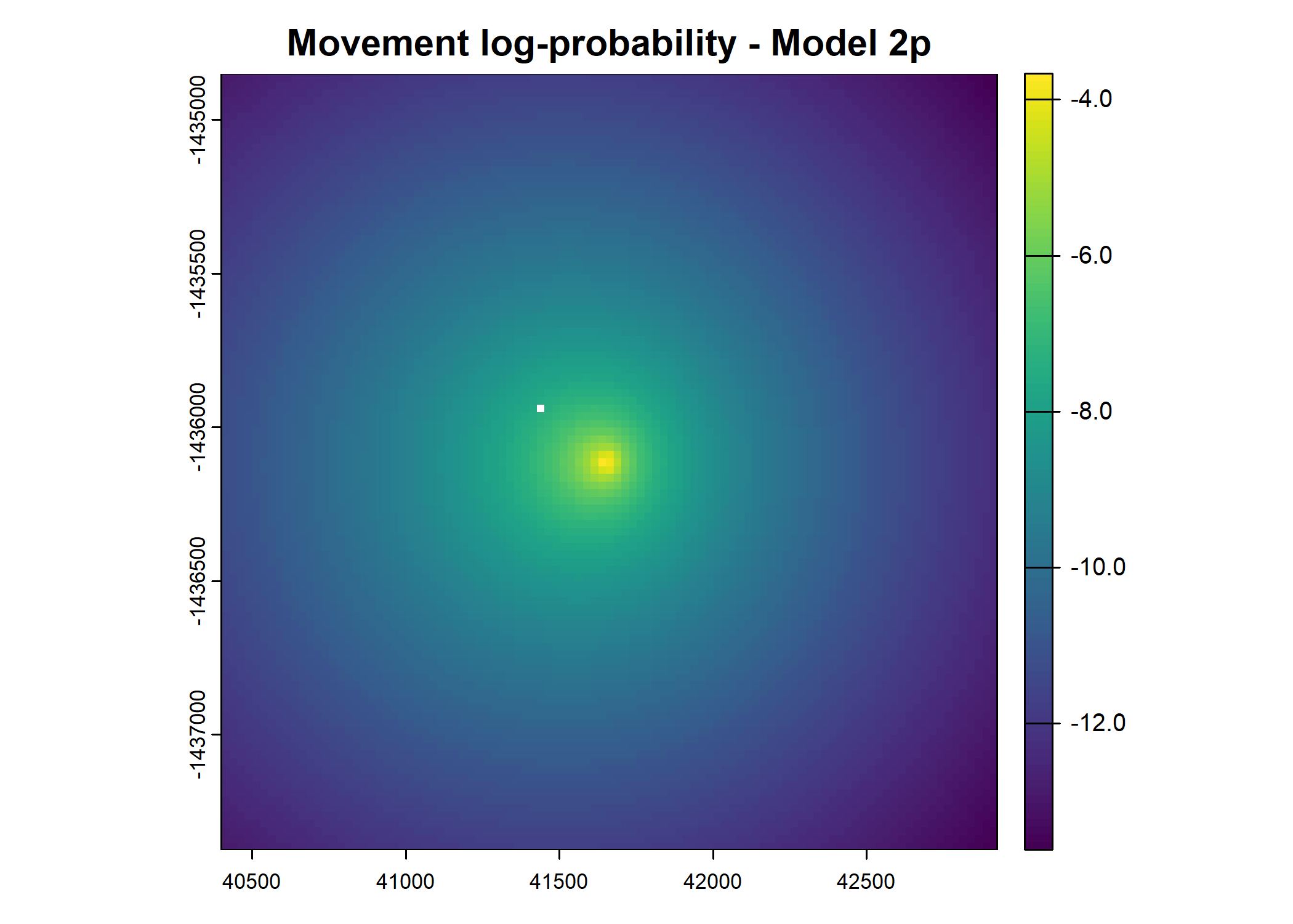
Movement Probability
- Step length is modeled via a Gamma distribution (using
shapeandscaleparameters). - Turning angle is modeled via the von Mises distribution (using
kappaand a mean angle based on the previous step’s bearing). - The log-probability of these components is combined (
move_log) and normalised.
- Step length is modeled via a Gamma distribution (using
Next-Step Probability
- The habitat and movement log-probabilities are summed to get the next-step log-probability.
- It is normalised to yield the next-step probability for each candidate pixel (where all pixels sum to 1).
- The script then extracts the probability at the buffalo’s actual next location (
prob_next_step_ssf_0porprob_next_step_ssf_2p).
Outputs
- For each step, the script appends probabilities (
prob_habitat_ssf_0/2p,prob_movement_ssf_0/2p, andprob_next_step_ssf_0/2p) to the data frame.
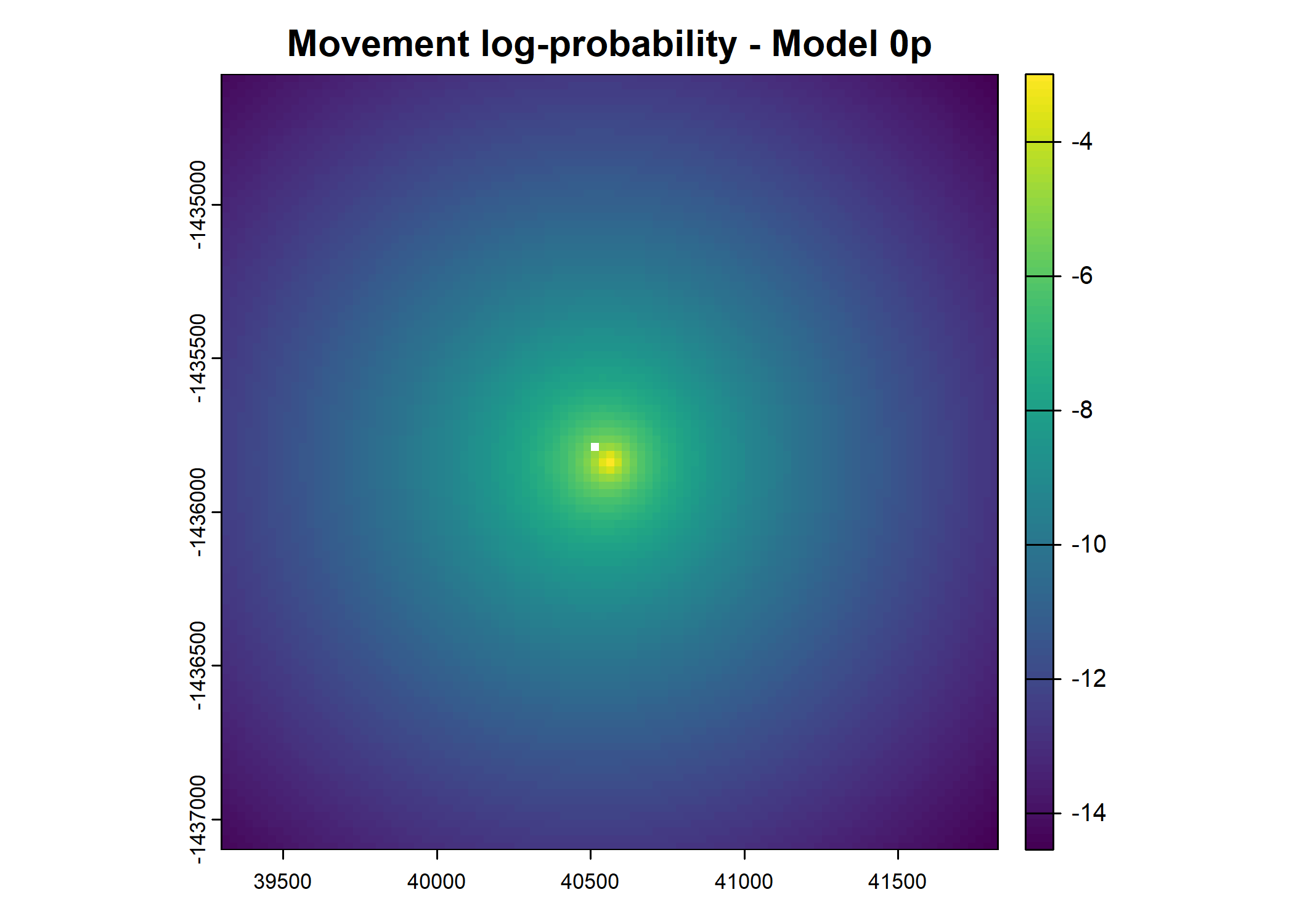
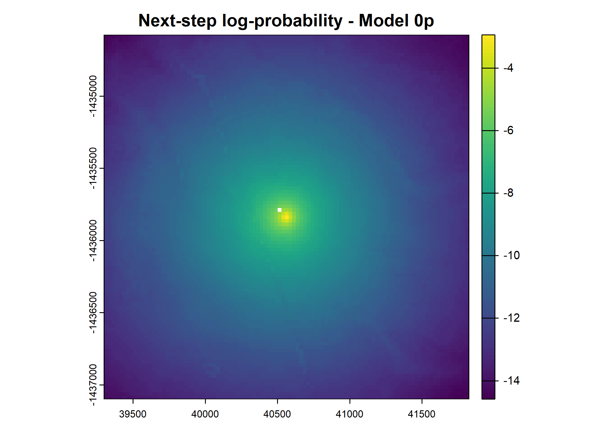
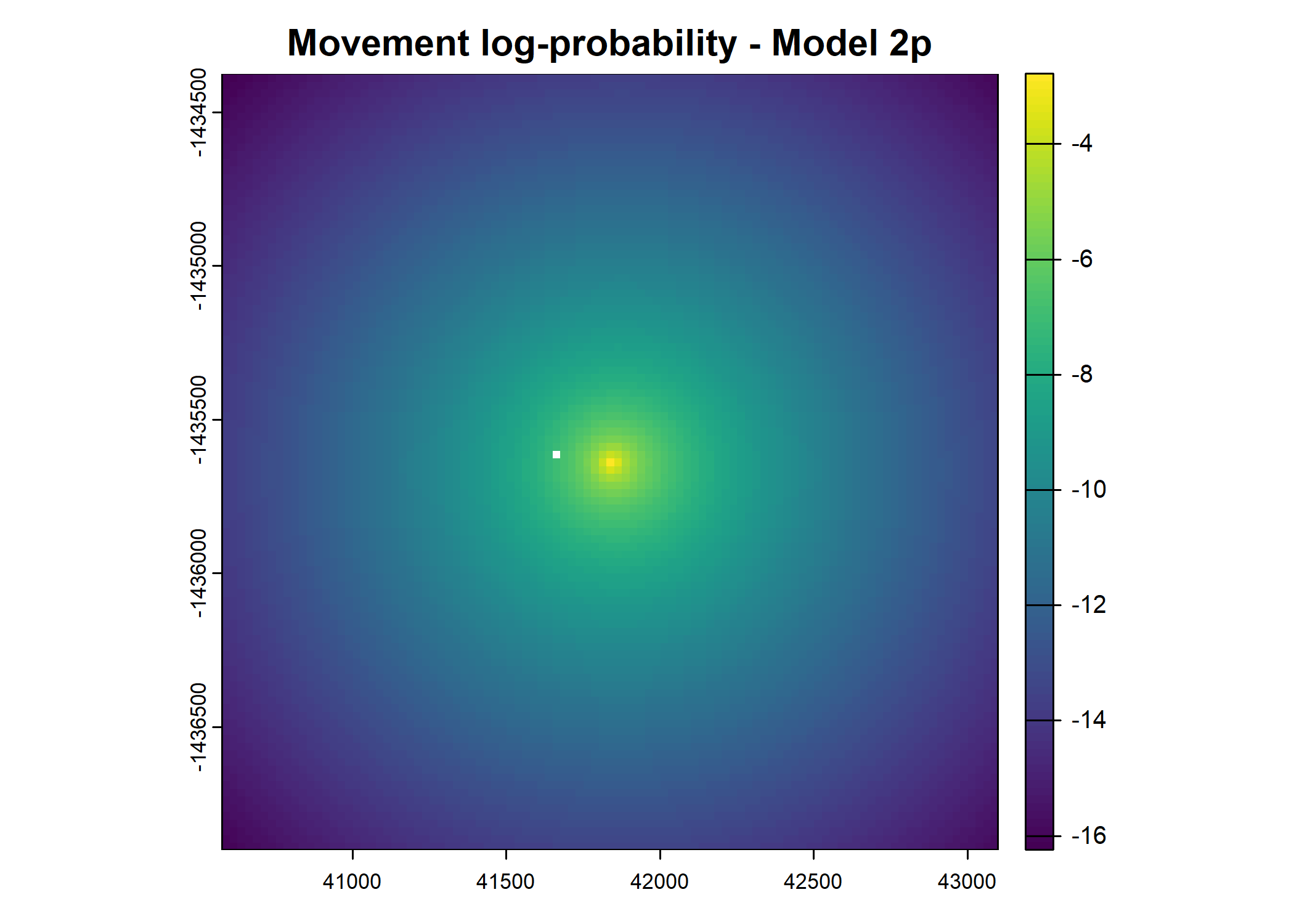
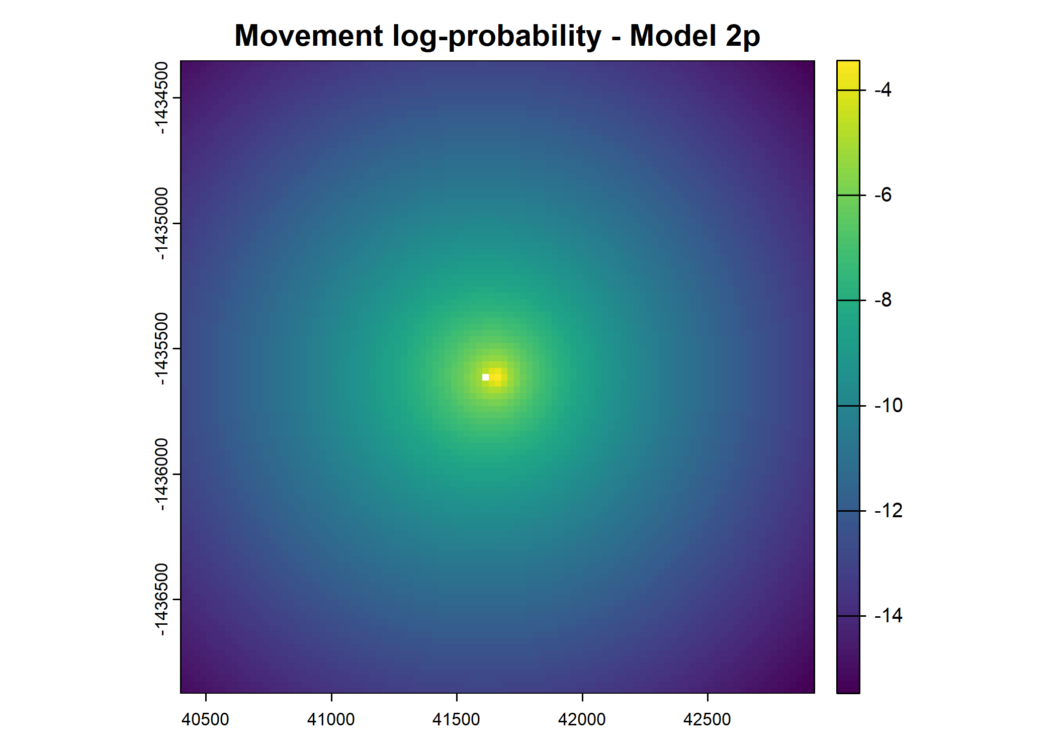
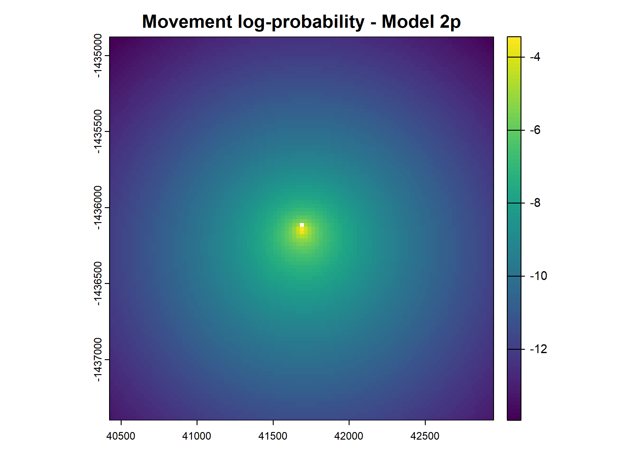
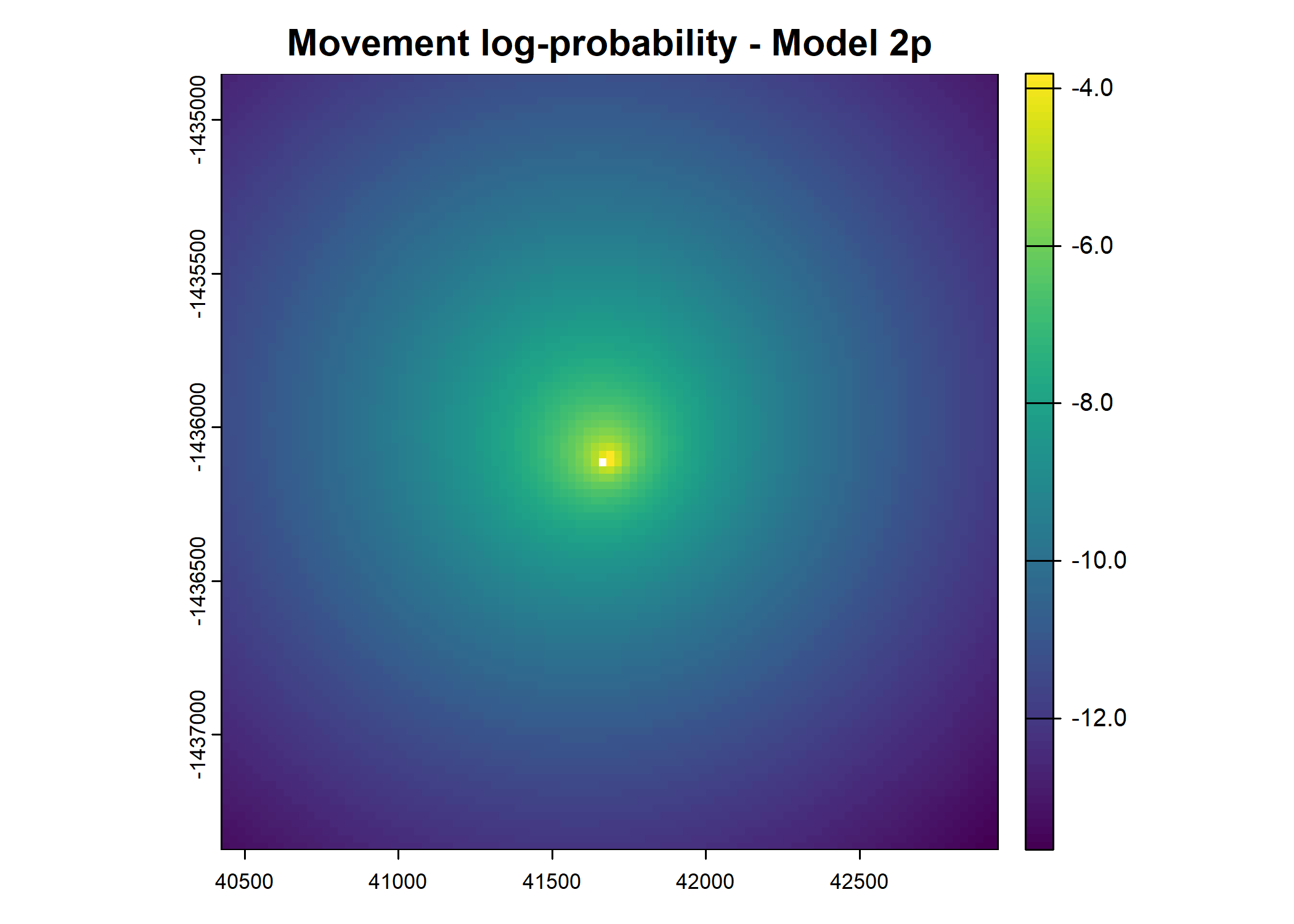
Diagnostic Plots
- For the first few steps of the first buffalo (which is the focal id), the script plots local covariate layers and the log-probability surfaces (habitat, movement, and combined next-step).
Code
#-------------------------------------------------------------------------
### Select a buffalo's data
#-------------------------------------------------------------------------
# for(k in 1:length(buffalo_id_list)) {
for(k in 1:1) {
data_id <- buffalo_id_list[[k]]
attr(data_id$t_, "tzone") <- "Australia/Queensland"
attr(data_id$t2_, "tzone") <- "Australia/Queensland"
data_id <- data_id %>% mutate(
year_t2 = year(t2_),
yday_t2_2018_base = ifelse(year_t2 == 2018, yday_t2, 365+yday_t2)
)
sample_extent <- 1250
# remove steps that fall outside of the local spatial extent
data_id <- data_id %>%
filter(x2_cent > -sample_extent &
x2_cent < sample_extent &
y2_cent > -sample_extent &
y2_cent < sample_extent) %>%
drop_na(ta)
# max(data_id$yday_t2_2018_base)
# write_csv(data_id, paste0("buffalo_local_data_id/validation/validation_", buffalo_data_ids[k]))
model_harmonics <- c("0p", "2p")
test_data <- data_id %>% slice(1:100) # test with a subset of the data
# test_data <- data_id
# subset rasters around all of the locations of the current buffalo (speeds up local subsetting)
buffer <- 2000
template_raster_crop <- terra::rast(xmin = min(test_data$x2_) - buffer,
xmax = max(test_data$x2_) + buffer,
ymin = min(test_data$y2_) - buffer,
ymax = max(test_data$y2_) + buffer,
resolution = 25,
crs = "epsg:3112")
## Crop the rasters
ndvi_projected_cropped <- terra::crop(ndvi_projected, template_raster_crop)
ndvi_projected_cropped_sq <- ndvi_projected_cropped^2
canopy_cover_cropped <- terra::crop(canopy_cover, template_raster_crop)
canopy01_cropped <- canopy_cover_cropped/100
canopy01_cropped_sq <- canopy01_cropped^2
veg_herby_cropped <- terra::crop(veg_herby, template_raster_crop)
slope_cropped <- terra::crop(slope, template_raster_crop)
tic()
#-------------------------------------------------------------------------
### Select a model (without temporal dynamics - 0p, or with temporal dynamics - 2p)
#-------------------------------------------------------------------------
for(j in 1:length(model_harmonics)) {
ssf_coefs_file_path <- paste0("ssf_coefficients/id", focal_id, "_", model_harmonics[j], "Daily_coefs_80-10-10_", model_date, ".csv")
print(ssf_coefs_file_path)
ssf_coefs <- read_csv(ssf_coefs_file_path)
# keep only the integer hours using the modulo operator
ssf_coefs <- ssf_coefs %>% filter(ssf_coefs$hour %% 1 == 0)
# for the progress bar - uncomment the line depending on if using subset
# for all data
n <- nrow(test_data)
# for the subset
# n <- n_samples_subset
pb <- progress_bar$new(
format = " Progress [:bar] :percent in :elapsed",
total = n,
clear = FALSE
)
tic()
#-------------------------------------------------------------------------
### Loop over every step in the trajectory
#-------------------------------------------------------------------------
# to calculate the next step probabilities for all samples
# for (i in 2:n) {
sample_plot <- 1
for (i in sample_plot:(sample_plot+10)) {
# for (i in sample_plot:sample_plot) {
# for the subset
# for (i in 2:(n_samples_subset+1)) {
sample_tm1 <- test_data[i-1, ] # get the step at t - 1 for the bearing of the approaching step
sample <- test_data[i, ]
sample_extent <- ext(sample$x_min, sample$x_max, sample$y_min, sample$y_max)
#-------------------------------------------------------------------------
### Extract local covariates
#-------------------------------------------------------------------------
# NDVI
ndvi_index <- which.min(abs(difftime(sample$t_, terra::time(ndvi_projected_cropped))))
ndvi_sample <- crop(ndvi_projected[[ndvi_index]], sample_extent)
# NDVI ^ 2
ndvi_sq_sample <- crop(ndvi_projected_cropped_sq[[ndvi_index]], sample_extent)
# Canopy cover
canopy_sample <- crop(canopy01_cropped, sample_extent)
# Canopy cover ^ 2
canopy_sq_sample <- crop(canopy01_cropped_sq, sample_extent)
# Herbaceous vegetation
veg_herby_sample <- crop(veg_herby_cropped, sample_extent)
# Slope
slope_sample <- crop(slope_cropped, sample_extent)
# create a SpatVector from the coordinates
next_step_vect <- vect(cbind(sample$x2_, sample$y2_), crs = crs(ndvi_sample))
#-------------------------------------------------------------------------
### calculate the next-step probability surfaces
#-------------------------------------------------------------------------
### Habitat selection probability
#-------------------------------------------------------------------------
# get the coefficients for the appropriate hour
coef_hour <- which(ssf_coefs$hour == sample$hour_t2)
# multiply covariate values by coefficients
# ndvi
ndvi_linear <- ndvi_sample * ssf_coefs$ndvi[[coef_hour]]
ndvi_quad <- ndvi_sq_sample * ssf_coefs$ndvi_2[[coef_hour]]
# canopy cover
canopy_linear <- canopy_sample * ssf_coefs$canopy[[coef_hour]]
canopy_quad <- canopy_sq_sample * ssf_coefs$canopy_2[[coef_hour]]
# veg_herby
veg_herby_pred <- veg_herby_sample * ssf_coefs$herby[[coef_hour]]
# slope
slope_pred <- slope_sample * ssf_coefs$slope[[coef_hour]]
# combining all covariates (on the log-scale)
habitat_log <- ndvi_linear + ndvi_quad + canopy_linear + canopy_quad + slope_pred + veg_herby_pred
# create template raster
habitat_pred <- habitat_log
# convert to normalised probability
habitat_pred[] <- exp(values(habitat_log) - max(values(habitat_log), na.rm = T)) /
sum(exp(values(habitat_log) - max(values(habitat_log), na.rm = T)), na.rm = T)
# print(sum(values(habitat_pred)))
# habitat probability value at the next step
prob_habitat <- as.numeric(terra::extract(habitat_pred, next_step_vect)[2])
# print(paste0("Habitat probability: ", prob_habitat))
### Movement Probability
#-------------------------------------------------------------------------
# step lengths
# calculated on the log scale
# subtract the log(distance values to account for the change in movement variables - Appendix in paper)
step_log <- habitat_log
step_log[] <- dgamma(distance_values,
shape = ssf_coefs$shape[[coef_hour]],
scale = ssf_coefs$scale[[coef_hour]], log = TRUE) - log(distance_values)
# normalise the step length probabilities
# step_log[] <- values(step_log) - max(values(step_log), na.rm = T) -
# log(sum(exp(values(step_log) - max(values(step_log), na.rm = T))))
# check that they sum to 1
# print(sum(exp(values(step_log))))
# turning angles
ta_log <- habitat_log
vm_mu <- sample$bearing
vm_mu_updated <- ifelse(ssf_coefs$kappa[[coef_hour]] > 0, sample_tm1$bearing, sample_tm1$bearing - pi)
ta_log[] <- suppressWarnings(circular::dvonmises(bearing_values,
mu = vm_mu_updated,
kappa = abs(ssf_coefs$kappa[[coef_hour]]),
log = TRUE))
# normalise the turning angle probabilities
# ta_log[] <- values(ta_log) - max(values(ta_log), na.rm = T) -
# log(sum(exp(values(ta_log) - max(values(ta_log), na.rm = T))))
# check that they sum to 1
# print(sum(exp(values(ta_log))))
# combine the step and turning angle probabilities
move_log <- step_log + ta_log
# create template raster
move_pred <- habitat_log
# convert to normalised probability
move_pred[] <- exp(values(move_log) - max(values(move_log), na.rm = T)) /
sum(exp(values(move_log) - max(values(move_log), na.rm = T)), na.rm = T)
# print(sum(values(move_pred)))
# movement probability value at the next step
prob_movement <- as.numeric(terra::extract(move_pred, next_step_vect)[2])
# print(prob_movement)
# Next-step probability
#-------------------------------------------------------------------------
# calculate the next-step log probability
next_step_log <- habitat_log + move_log
# create template raster
next_step_pred <- habitat_log
# normalise using log-sum-exp trick
next_step_pred[] <- exp(values(next_step_log) - max(values(next_step_log), na.rm = T)) /
sum(exp(values(next_step_log) - max(values(next_step_log), na.rm = T)), na.rm = T)
# print(sum(values(next_step_pred)))
# check next-step location
next_step_sample <- terra::mask(next_step_pred, next_step_vect, inverse = T)
# plot(next_step_sample)
# check which cell is NA in rows and columns
# print(rowColFromCell(next_step_pred, which(is.na(values(next_step_sample)))))
# NDVI value at next step (to check against the deepSSF version)
# ndvi_next_step <- as.numeric(terra::extract(ndvi_sample, next_step_vect)[2])
# print(paste("NDVI value = ", ndvi_next_step))
# next-step probability value at the next step
prob_next_step <- as.numeric(terra::extract(next_step_pred, next_step_vect)[2])
# print(prob_next_step)
test_data[i, paste0("prob_habitat_ssf_", model_harmonics[j])] <- prob_habitat
test_data[i, paste0("prob_movement_ssf_", model_harmonics[j])] <- prob_movement
test_data[i, paste0("prob_next_step_ssf_", model_harmonics[j])] <- prob_next_step
# plot a few local covariates and the predictions for the focal buffalo
# if(k == 1 & i < 7){
if(k == 1){
print(sample)
png(paste0("outputs/next_step_validation/ndvi_step_", i, ".png"),
width = 800, height = 750, res = 150)
plot(ndvi_sample, main = "NDVI")
dev.off()
png(paste0("outputs/next_step_validation/canopy_", i, ".png"),
width = 800, height = 750, res = 150)
plot(canopy_sample, main = "Canopy cover")
dev.off()
png(paste0("outputs/next_step_validation/herby_", i, ".png"),
width = 800, height = 750, res = 150)
plot(veg_herby_sample, main = "Herbaceous vegetation")
dev.off()
png(paste0("outputs/next_step_validation/slope_", i, ".png"),
width = 800, height = 750, res = 150)
plot(slope_sample, main = "Slope")
dev.off()
png(paste0("outputs/next_step_validation/habitat_log_step_", i, "_model_", j, ".png"),
width = 800, height = 750, res = 150)
plot(terra::mask(log(habitat_pred), next_step_vect, inverse = T),
main = paste0("Habitat selection (log) - Model ", model_harmonics[j]))
# plot(habitat_pred)
dev.off()
png(paste0("outputs/next_step_validation/habitat_step_", i, "_model_", j, ".png"),
width = 800, height = 750, res = 150)
plot(terra::mask(habitat_pred, next_step_vect, inverse = T),
main = paste0("Habitat selection - Model ", model_harmonics[j]))
dev.off()
# plot(step_log, main = "")
# plot(ta_log, main = "")
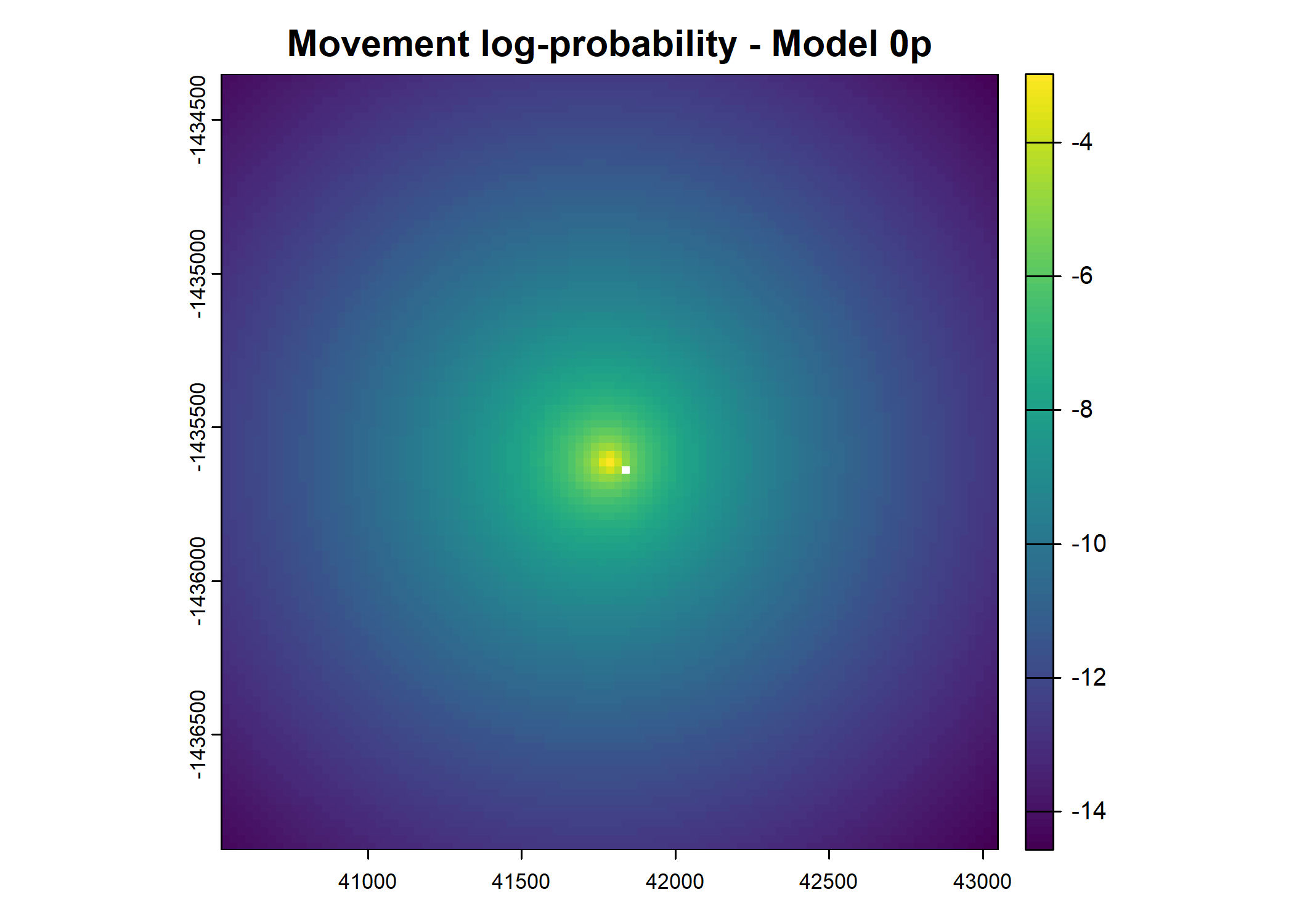
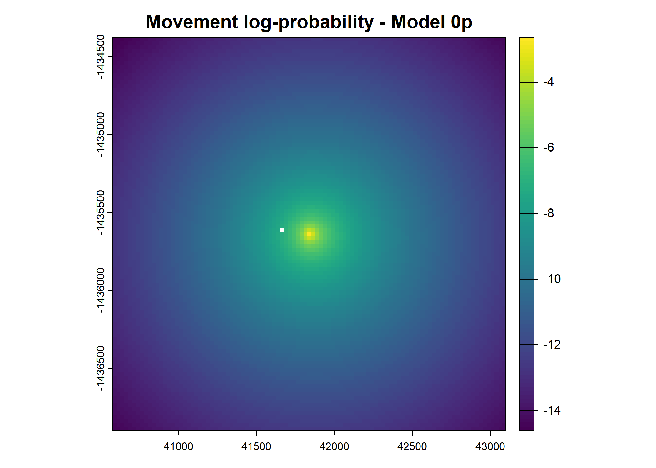
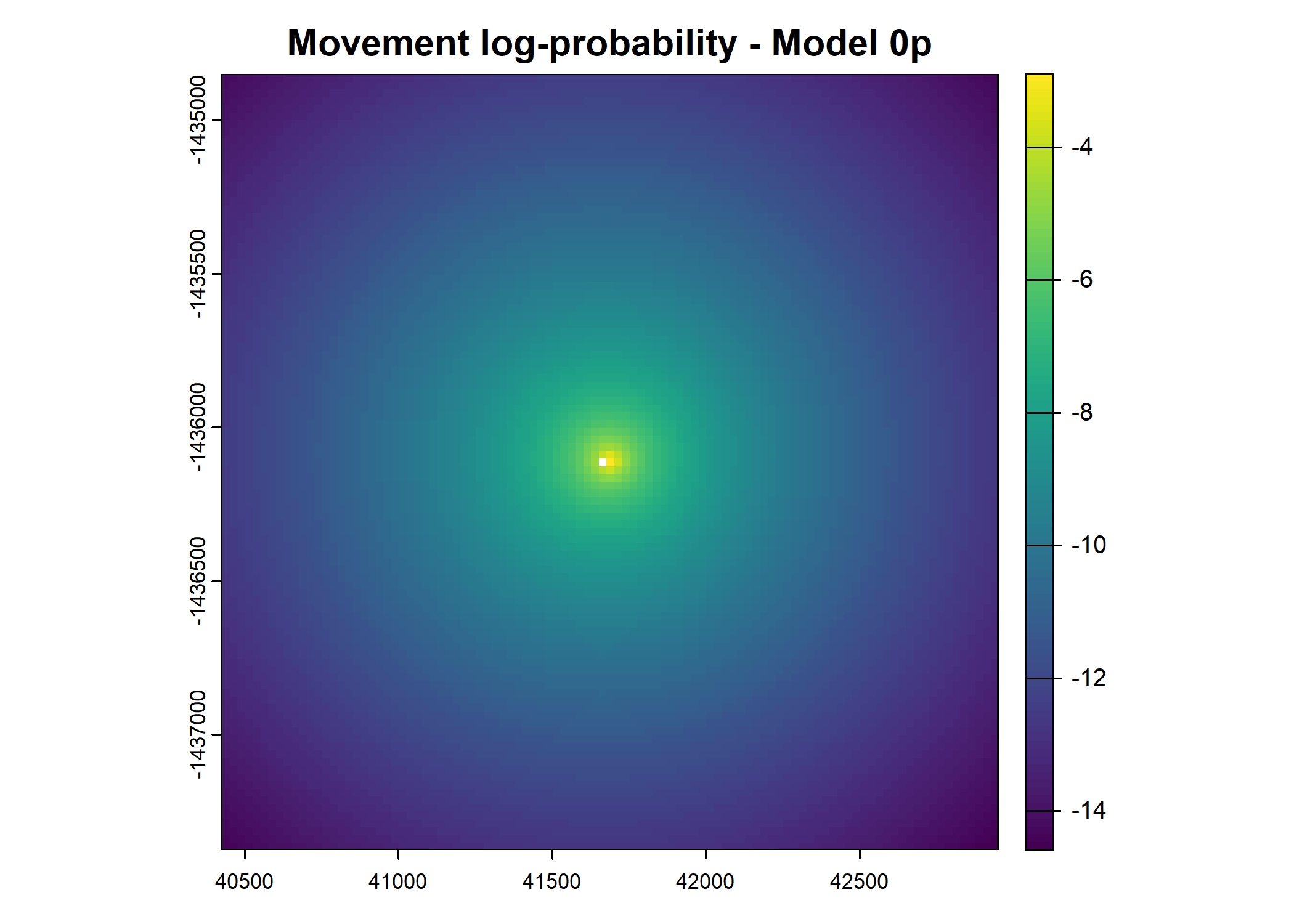
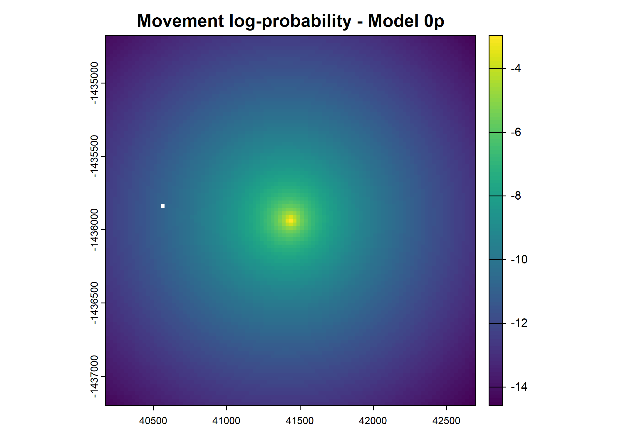
plot(terra::mask(log(move_pred), next_step_vect, inverse = T),
main = paste0("Movement log-probability - Model ", model_harmonics[j]))
# plot(move_pred)
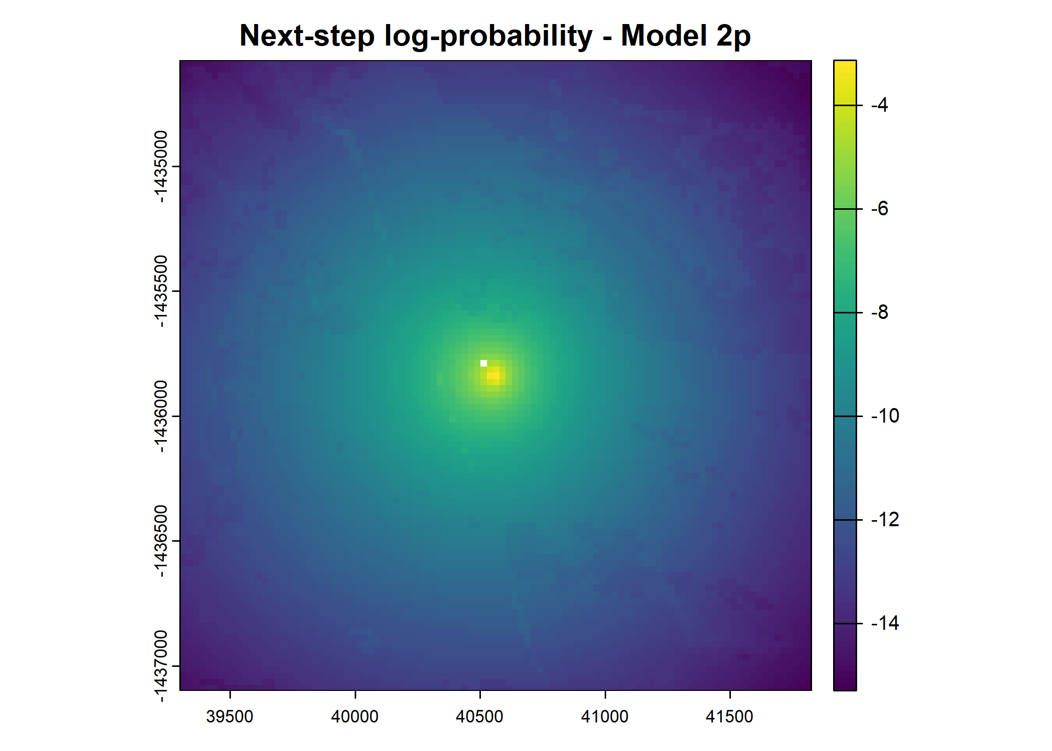
plot(terra::mask(log(next_step_pred), next_step_vect, inverse = T),
main = paste0("Next-step log-probability - Model ", model_harmonics[j]))
# plot(next_step_pred)
}
pb$tick() # Update progress bar
}
toc()
}
# write.csv(test_data, file = paste0("outputs/next_step_validation/next_step_probs_ssf_80-10-10_id", ids[k], "_n_samples", n, "_", Sys.Date(), ".csv"))
gc()
}[1] "ssf_coefficients/id2005_0pDaily_coefs_80-10-10_2025-04-10.csv"Rows: 240 Columns: 13
── Column specification ────────────────────────────────────────────────────────
Delimiter: ","
dbl (13): hour, ndvi, ndvi_2, canopy, canopy_2, slope, herby, sl, log_sl, co...
ℹ Use `spec()` to retrieve the full column specification for this data.
ℹ Specify the column types or set `show_col_types = FALSE` to quiet this message.Warning in max(values(move_log), na.rm = T): no non-missing arguments to max;
returning -Inf
Warning in max(values(move_log), na.rm = T): no non-missing arguments to max;
returning -InfWarning in max(values(next_step_log), na.rm = T): no non-missing arguments to
max; returning -Inf
Warning in max(values(next_step_log), na.rm = T): no non-missing arguments to
max; returning -InfWarning: Failed to compute min/max, no valid pixels found in sampling. (GDAL
error 1) x_ y_ t_ id x1_ y1_ x2_
1 41969.31 -1435671 2018-07-25T01:04:23Z 2005 41969.31 -1435671 41921.52
y2_ x2_cent y2_cent t2_ t_diff hour_t1 yday_t1
1 -1435654 -47.78894 16.85711 2018-07-25T02:04:39Z 1 11 206
hour_t2 hour_t2_sin hour_t2_cos yday_t2 yday_t2_sin yday_t2_cos sl
1 12 1.224606e-16 -1 206 -0.3913578 -0.9202386 50.67489
log_sl bearing bearing_sin bearing_cos ta cos_ta x_min x_max
1 3.925431 2.802478 0.3326521 -0.9430496 1.367942 0.201466 40706.81 43231.81
y_min y_max s2_index points_vect_cent year_t2 yday_t2_2018_base
1 -1436934 -1434409 7 NA 2018 206Warning: Failed to compute min/max, no valid pixels found in sampling. (GDAL
error 1)
Warning: Failed to compute min/max, no valid pixels found in sampling. (GDAL
error 1)
x_ y_ t_ id x1_ y1_ x2_
2 41921.52 -1435654 2018-07-25T02:04:39Z 2005 41921.52 -1435654 41779.44
y2_ x2_cent y2_cent t2_ t_diff hour_t1 yday_t1
2 -1435601 -142.0823 53.56843 2018-07-25T03:04:17Z 1 12 206
hour_t2 hour_t2_sin hour_t2_cos yday_t2 yday_t2_sin yday_t2_cos sl
2 13 -0.258819 -0.9659258 206 -0.3913578 -0.9202386 151.8452
log_sl bearing bearing_sin bearing_cos ta cos_ta x_min
2 5.022862 2.781049 0.3527831 -0.9357051 -0.02142933 0.9997704 40659.02
x_max y_min y_max s2_index points_vect_cent year_t2
2 43184.02 -1436917 -1434392 7 NA 2018
yday_t2_2018_base prob_habitat_ssf_0p prob_movement_ssf_0p
2 206 NA NA
prob_next_step_ssf_0p
2 NA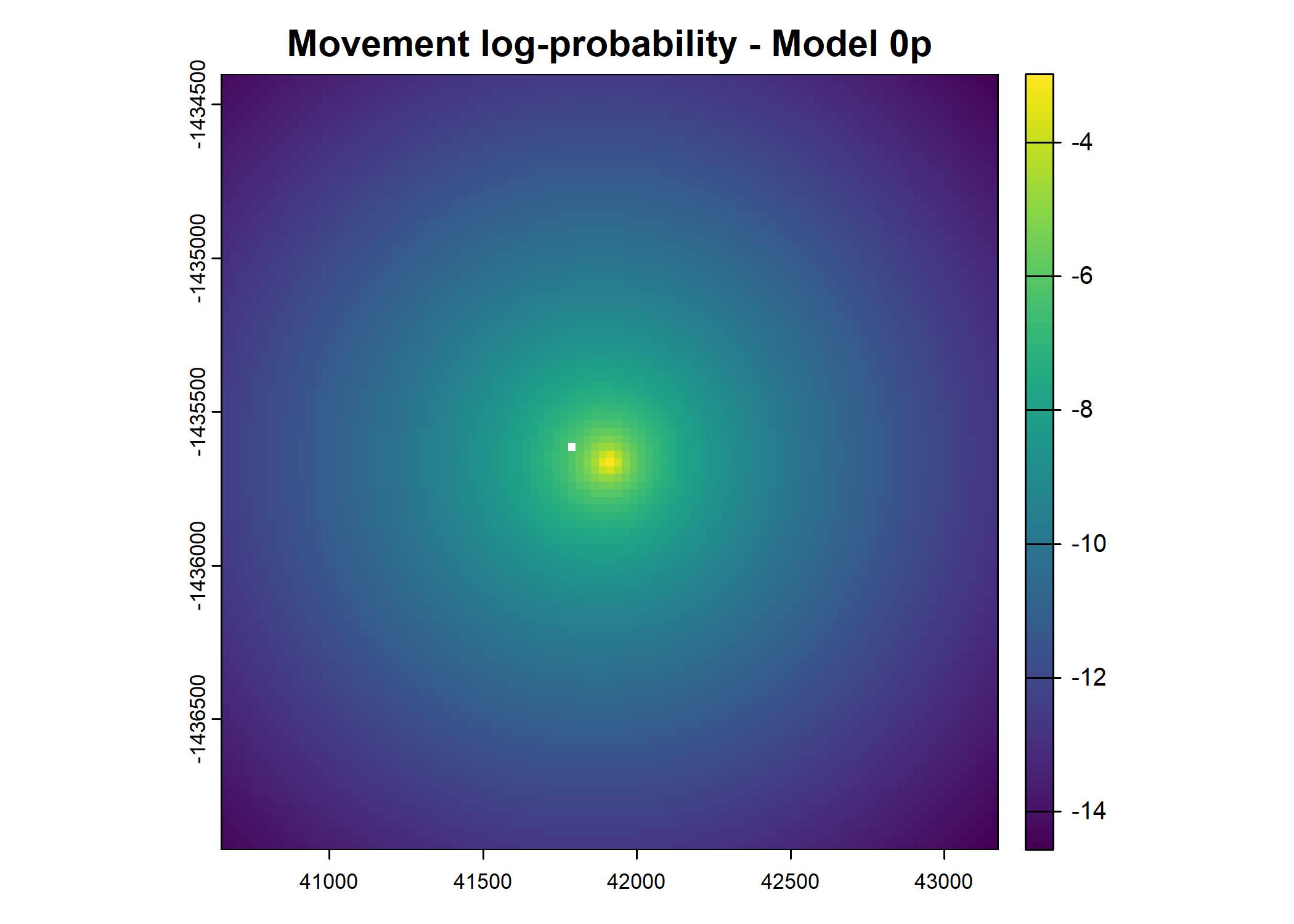
x_ y_ t_ id x1_ y1_ x2_
3 41779.44 -1435601 2018-07-25T03:04:17Z 2005 41779.44 -1435601 41841.2
y2_ x2_cent y2_cent t2_ t_diff hour_t1 yday_t1
3 -1435635 61.76368 -34.32294 2018-07-25T04:04:39Z 1 13 206
hour_t2 hour_t2_sin hour_t2_cos yday_t2 yday_t2_sin yday_t2_cos sl
3 14 -0.5 -0.8660254 206 -0.3913578 -0.9202386 70.65986
log_sl bearing bearing_sin bearing_cos ta cos_ta x_min
3 4.257878 -0.5072195 -0.4857487 0.8740985 2.994917 -0.9892624 40516.94
x_max y_min y_max s2_index points_vect_cent year_t2
3 43041.94 -1436863 -1434338 7 NA 2018
yday_t2_2018_base prob_habitat_ssf_0p prob_movement_ssf_0p
3 206 NA NA
prob_next_step_ssf_0p
3 NA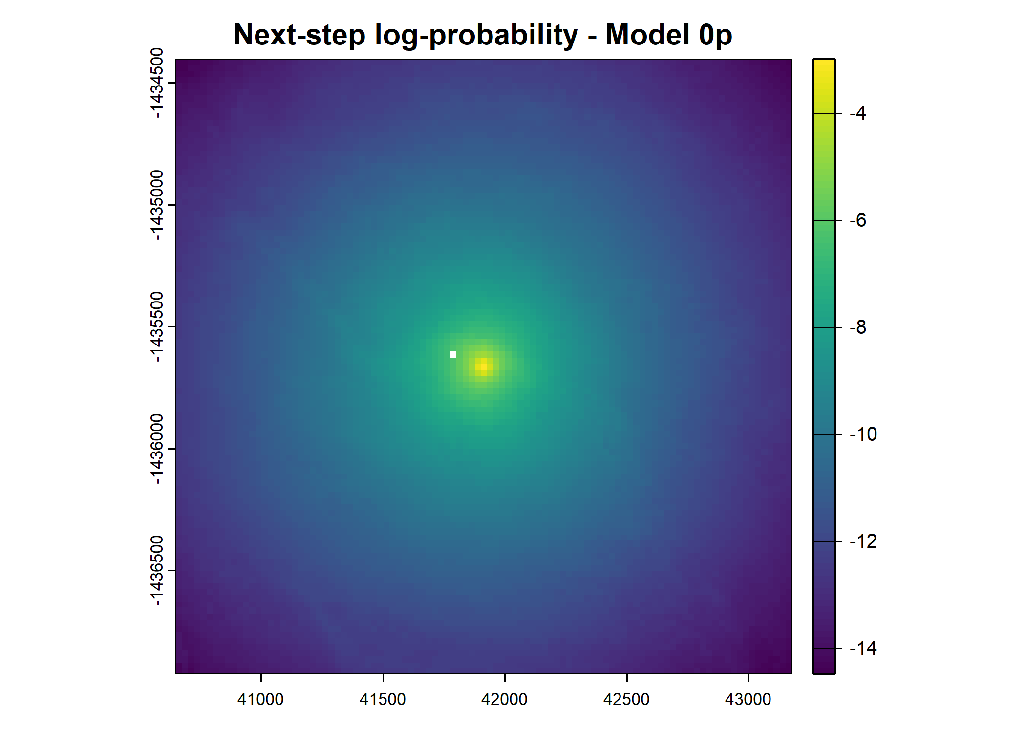
x_ y_ t_ id x1_ y1_ x2_ y2_
4 41841.2 -1435635 2018-07-25T04:04:39Z 2005 41841.2 -1435635 41655.46 -1435604
x2_cent y2_cent t2_ t_diff hour_t1 yday_t1 hour_t2
4 -185.7399 31.00353 2018-07-25T05:04:27Z 1 14 206 15
hour_t2_sin hour_t2_cos yday_t2 yday_t2_sin yday_t2_cos sl log_sl
4 -0.7071068 -0.7071068 206 -0.3913578 -0.9202386 188.3097 5.238088
bearing bearing_sin bearing_cos ta cos_ta x_min x_max
4 2.976198 0.1646412 -0.9863535 -2.799767 -0.9421444 40578.7 43103.7
y_min y_max s2_index points_vect_cent year_t2 yday_t2_2018_base
4 -1436898 -1434373 7 NA 2018 206
prob_habitat_ssf_0p prob_movement_ssf_0p prob_next_step_ssf_0p
4 NA NA NA
x_ y_ t_ id x1_ y1_ x2_
5 41655.46 -1435604 2018-07-25T05:04:27Z 2005 41655.46 -1435604 41618.65
y2_ x2_cent y2_cent t2_ t_diff hour_t1 yday_t1
5 -1435608 -36.81141 -4.438037 2018-07-25T06:04:24Z 1 15 206
hour_t2 hour_t2_sin hour_t2_cos yday_t2 yday_t2_sin yday_t2_cos sl
5 16 -0.8660254 -0.5 206 -0.3913578 -0.9202386 37.07797
log_sl bearing bearing_sin bearing_cos ta cos_ta x_min
5 3.613023 -3.02161 -0.1196947 -0.9928107 0.2853766 0.9595557 40392.96
x_max y_min y_max s2_index points_vect_cent year_t2
5 42917.96 -1436867 -1434342 7 NA 2018
yday_t2_2018_base prob_habitat_ssf_0p prob_movement_ssf_0p
5 206 NA NA
prob_next_step_ssf_0p
5 NA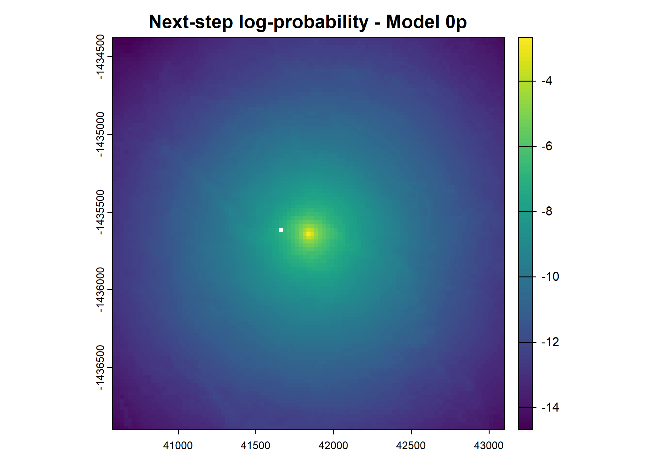

x_ y_ t_ id x1_ y1_ x2_
6 41618.65 -1435608 2018-07-25T06:04:24Z 2005 41618.65 -1435608 41688.44
y2_ x2_cent y2_cent t2_ t_diff hour_t1 yday_t1
6 -1436126 69.78648 -517.1566 2018-07-25T07:04:28Z 1 16 206
hour_t2 hour_t2_sin hour_t2_cos yday_t2 yday_t2_sin yday_t2_cos sl
6 17 -0.9659258 -0.258819 206 -0.3913578 -0.9202386 521.8439
log_sl bearing bearing_sin bearing_cos ta cos_ta x_min
6 6.257369 -1.436664 -0.9910177 0.1337306 1.584946 -0.01414957 40356.15
x_max y_min y_max s2_index points_vect_cent year_t2
6 42881.15 -1436871 -1434346 7 NA 2018
yday_t2_2018_base prob_habitat_ssf_0p prob_movement_ssf_0p
6 206 NA NA
prob_next_step_ssf_0p
6 NA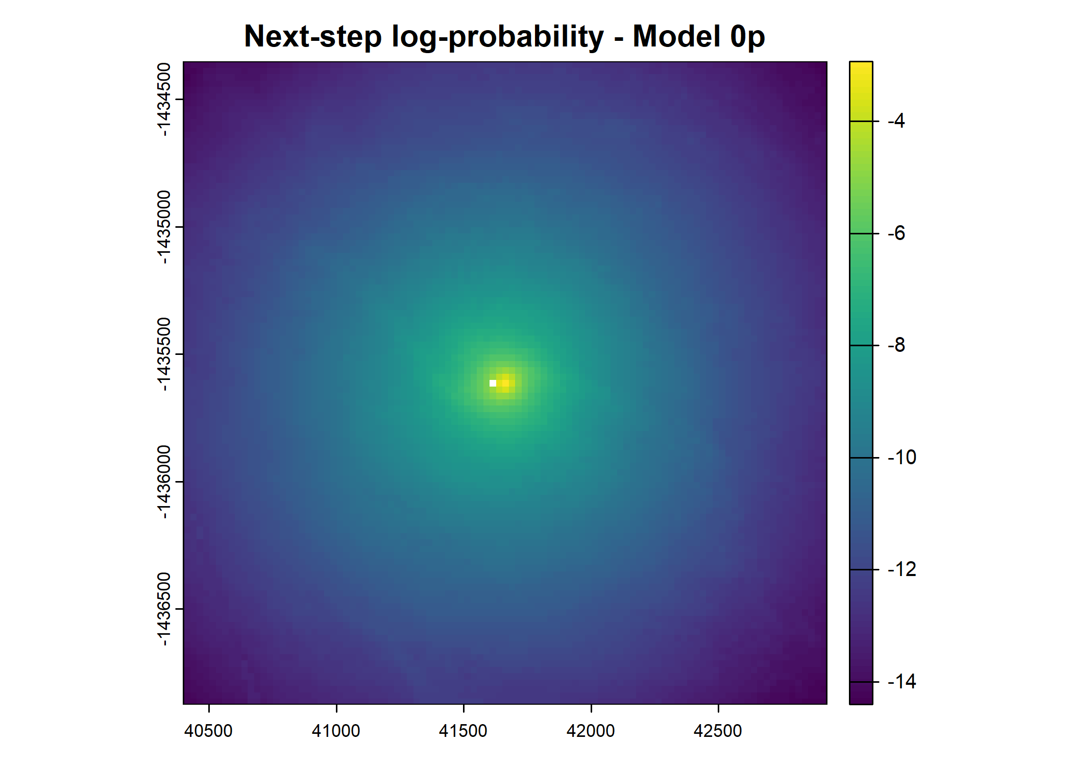

x_ y_ t_ id x1_ y1_ x2_
7 41688.44 -1436126 2018-07-25T07:04:28Z 2005 41688.44 -1436126 41684.34
y2_ x2_cent y2_cent t2_ t_diff hour_t1 yday_t1
7 -1436119 -4.095906 7.020228 2018-07-25T08:04:31Z 1 17 206
hour_t2 hour_t2_sin hour_t2_cos yday_t2 yday_t2_sin yday_t2_cos sl
7 18 -1 -1.83691e-16 206 -0.3913578 -0.9202386 8.127733
log_sl bearing bearing_sin bearing_cos ta cos_ta x_min
7 2.095282 2.098953 0.8637375 -0.503942 -2.747568 -0.9233716 40425.94
x_max y_min y_max s2_index points_vect_cent year_t2
7 42950.94 -1437388 -1434863 7 NA 2018
yday_t2_2018_base prob_habitat_ssf_0p prob_movement_ssf_0p
7 206 NA NA
prob_next_step_ssf_0p
7 NA

x_ y_ t_ id x1_ y1_ x2_
8 41684.34 -1436119 2018-07-25T08:04:31Z 2005 41684.34 -1436119 41674.59
y2_ x2_cent y2_cent t2_ t_diff hour_t1 yday_t1
8 -1436119 -9.754289 -0.08369654 2018-07-25T09:04:33Z 1 18 206
hour_t2 hour_t2_sin hour_t2_cos yday_t2 yday_t2_sin yday_t2_cos sl
8 19 -0.9659258 0.258819 206 -0.3913578 -0.9202386 9.754648
log_sl bearing bearing_sin bearing_cos ta cos_ta x_min
8 2.277744 -3.133012 -0.00858017 -0.9999632 1.05122 0.4965124 40421.84
x_max y_min y_max s2_index points_vect_cent year_t2
8 42946.84 -1437381 -1434856 7 NA 2018
yday_t2_2018_base prob_habitat_ssf_0p prob_movement_ssf_0p
8 206 NA NA
prob_next_step_ssf_0p
8 NA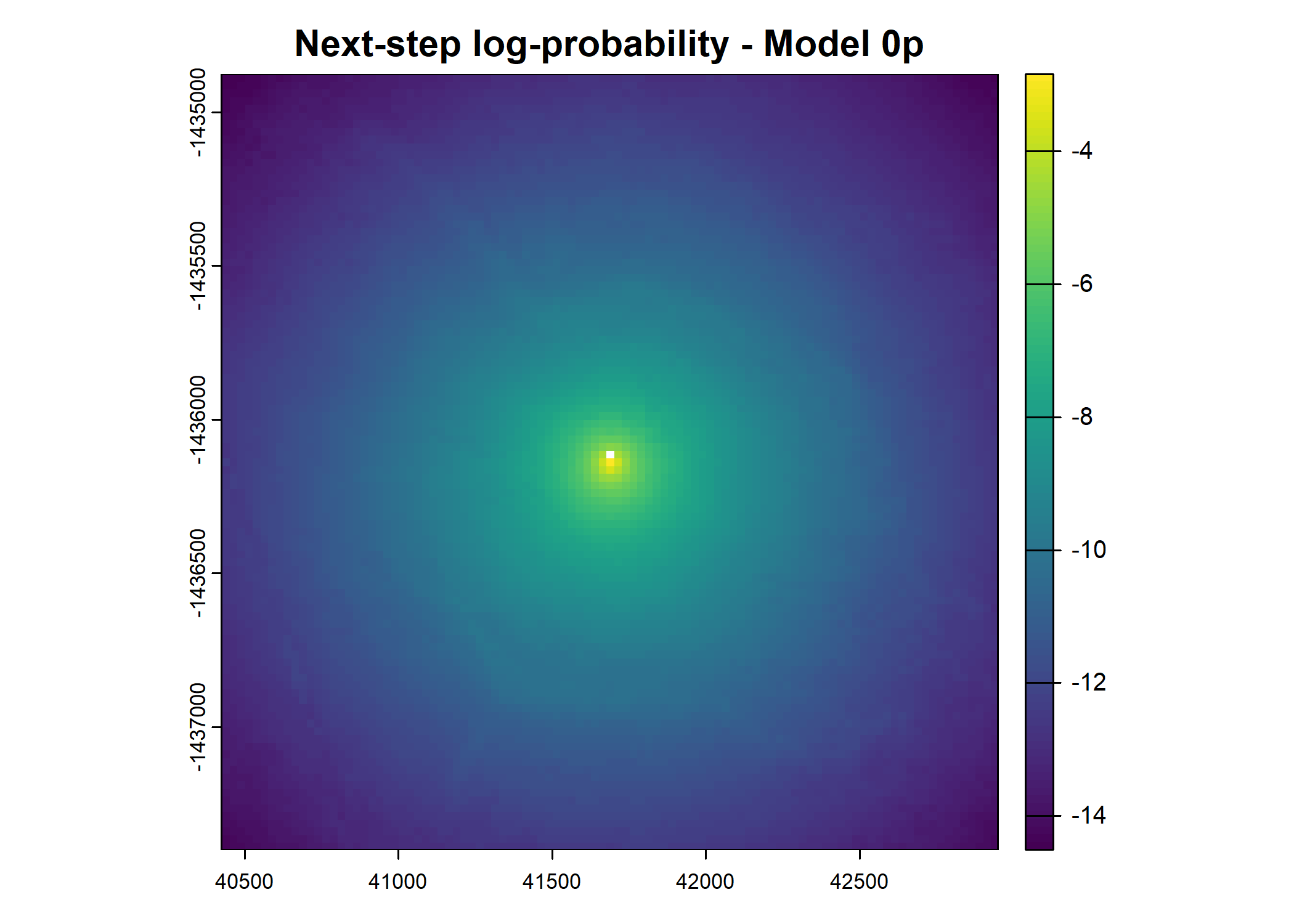
x_ y_ t_ id x1_ y1_ x2_
9 41674.59 -1436119 2018-07-25T09:04:33Z 2005 41674.59 -1436119 41425.16
y2_ x2_cent y2_cent t2_ t_diff hour_t1 yday_t1
9 -1435938 -249.4296 180.3333 2018-07-25T10:04:02Z 1 19 206
hour_t2 hour_t2_sin hour_t2_cos yday_t2 yday_t2_sin yday_t2_cos sl
9 20 -0.8660254 0.5 206 -0.3913578 -0.9202386 307.7908
log_sl bearing bearing_sin bearing_cos ta cos_ta x_min
9 5.72942 2.515608 0.5858955 -0.8103866 -0.6345649 0.8053297 40412.09
x_max y_min y_max s2_index points_vect_cent year_t2
9 42937.09 -1437381 -1434856 7 NA 2018
yday_t2_2018_base prob_habitat_ssf_0p prob_movement_ssf_0p
9 206 NA NA
prob_next_step_ssf_0p
9 NA

x_ y_ t_ id x1_ y1_ x2_
10 41425.16 -1435938 2018-07-25T10:04:02Z 2005 41425.16 -1435938 40563.21
y2_ x2_cent y2_cent t2_ t_diff hour_t1 yday_t1
10 -1435841 -861.9445 97.45269 2018-07-25T11:04:04Z 1 20 206
hour_t2 hour_t2_sin hour_t2_cos yday_t2 yday_t2_sin yday_t2_cos sl
10 21 -0.7071068 0.7071068 206 -0.3913578 -0.9202386 867.4361
log_sl bearing bearing_sin bearing_cos ta cos_ta x_min
10 6.765542 3.029009 0.1123457 -0.9936692 0.5134012 0.8710791 40162.66
x_max y_min y_max s2_index points_vect_cent year_t2
10 42687.66 -1437201 -1434676 7 NA 2018
yday_t2_2018_base prob_habitat_ssf_0p prob_movement_ssf_0p
10 206 NA NA
prob_next_step_ssf_0p
10 NA
x_ y_ t_ id x1_ y1_ x2_
11 40563.21 -1435841 2018-07-25T11:04:04Z 2005 40563.21 -1435841 40512.76
y2_ x2_cent y2_cent t2_ t_diff hour_t1 yday_t1
11 -1435777 -50.44988 63.87376 2018-07-25T12:05:13Z 1 21 206
hour_t2 hour_t2_sin hour_t2_cos yday_t2 yday_t2_sin yday_t2_cos sl
11 22 -0.5 0.8660254 206 -0.3913578 -0.9202386 81.39439
log_sl bearing bearing_sin bearing_cos ta cos_ta x_min
11 4.399306 2.23931 0.784744 -0.61982 -0.7896996 0.7040587 39300.71
x_max y_min y_max s2_index points_vect_cent year_t2
11 41825.71 -1437103 -1434578 7 NA 2018
yday_t2_2018_base prob_habitat_ssf_0p prob_movement_ssf_0p
11 206 NA NA
prob_next_step_ssf_0p
11 NA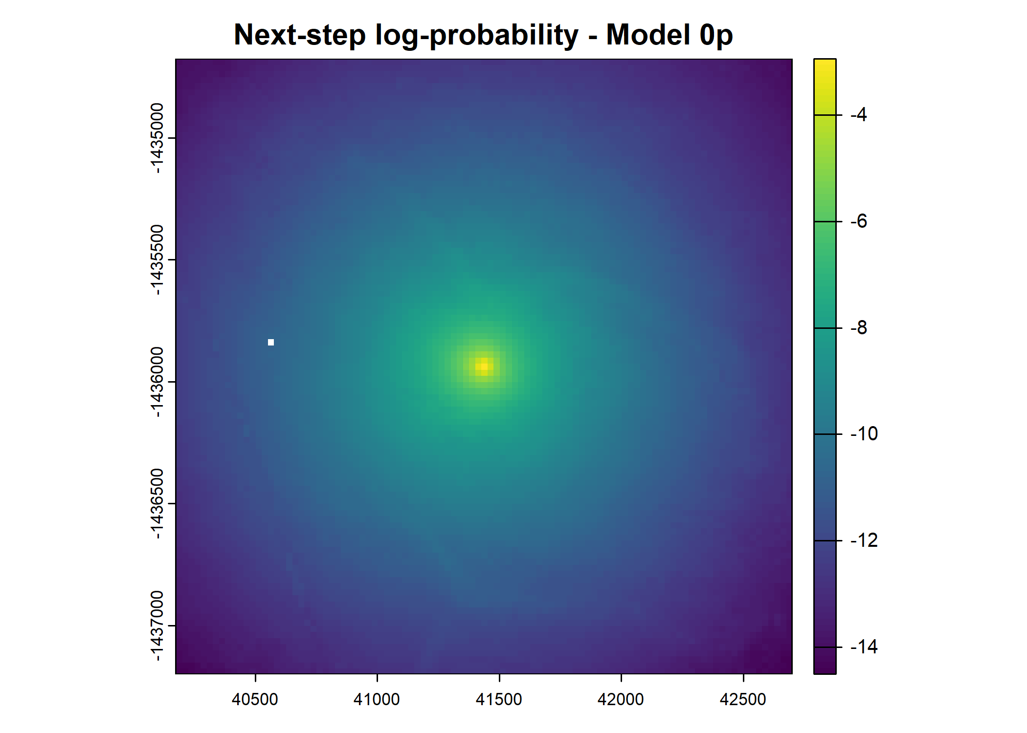
41.44 sec elapsed
[1] "ssf_coefficients/id2005_2pDaily_coefs_80-10-10_2025-04-10.csv"Rows: 240 Columns: 13
── Column specification ────────────────────────────────────────────────────────
Delimiter: ","
dbl (13): hour, ndvi, ndvi_2, canopy, canopy_2, slope, herby, sl, log_sl, co...
ℹ Use `spec()` to retrieve the full column specification for this data.
ℹ Specify the column types or set `show_col_types = FALSE` to quiet this message.Warning in max(values(move_log), na.rm = T): no non-missing arguments to max;
returning -InfWarning in max(values(move_log), na.rm = T): no non-missing arguments to max;
returning -InfWarning in max(values(next_step_log), na.rm = T): no non-missing arguments to
max; returning -Inf
Warning in max(values(next_step_log), na.rm = T): no non-missing arguments to
max; returning -InfWarning: Failed to compute min/max, no valid pixels found in sampling. (GDAL
error 1) x_ y_ t_ id x1_ y1_ x2_
1 41969.31 -1435671 2018-07-25T01:04:23Z 2005 41969.31 -1435671 41921.52
y2_ x2_cent y2_cent t2_ t_diff hour_t1 yday_t1
1 -1435654 -47.78894 16.85711 2018-07-25T02:04:39Z 1 11 206
hour_t2 hour_t2_sin hour_t2_cos yday_t2 yday_t2_sin yday_t2_cos sl
1 12 1.224606e-16 -1 206 -0.3913578 -0.9202386 50.67489
log_sl bearing bearing_sin bearing_cos ta cos_ta x_min x_max
1 3.925431 2.802478 0.3326521 -0.9430496 1.367942 0.201466 40706.81 43231.81
y_min y_max s2_index points_vect_cent year_t2 yday_t2_2018_base
1 -1436934 -1434409 7 NA 2018 206
prob_habitat_ssf_0p prob_movement_ssf_0p prob_next_step_ssf_0p
1 9.615473e-05 NA NAWarning: Failed to compute min/max, no valid pixels found in sampling. (GDAL
error 1)
Warning: Failed to compute min/max, no valid pixels found in sampling. (GDAL
error 1) x_ y_ t_ id x1_ y1_ x2_
2 41921.52 -1435654 2018-07-25T02:04:39Z 2005 41921.52 -1435654 41779.44
y2_ x2_cent y2_cent t2_ t_diff hour_t1 yday_t1
2 -1435601 -142.0823 53.56843 2018-07-25T03:04:17Z 1 12 206
hour_t2 hour_t2_sin hour_t2_cos yday_t2 yday_t2_sin yday_t2_cos sl
2 13 -0.258819 -0.9659258 206 -0.3913578 -0.9202386 151.8452
log_sl bearing bearing_sin bearing_cos ta cos_ta x_min
2 5.022862 2.781049 0.3527831 -0.9357051 -0.02142933 0.9997704 40659.02
x_max y_min y_max s2_index points_vect_cent year_t2
2 43184.02 -1436917 -1434392 7 NA 2018
yday_t2_2018_base prob_habitat_ssf_0p prob_movement_ssf_0p
2 206 9.65375e-05 0.001913733
prob_next_step_ssf_0p prob_habitat_ssf_2p prob_movement_ssf_2p
2 0.001924442 NA NA
prob_next_step_ssf_2p
2 NA
        x_       y_                   t_   id      x1_      y1_     x2_
3 41779.44 -1435601 2018-07-25T03:04:17Z 2005 41779.44 -1435601 41841.2
       y2_  x2_cent   y2_cent                  t2_ t_diff hour_t1 yday_t1
3 -1435635 61.76368 -34.32294 2018-07-25T04:04:39Z      1      13     206
  hour_t2 hour_t2_sin hour_t2_cos yday_t2 yday_t2_sin yday_t2_cos       sl
3      14        -0.5  -0.8660254     206  -0.3913578  -0.9202386 70.65986
    log_sl    bearing bearing_sin bearing_cos       ta     cos_ta    x_min
3 4.257878 -0.5072195  -0.4857487   0.8740985 2.994917 -0.9892624 40516.94
     x_max    y_min    y_max s2_index points_vect_cent year_t2
3 43041.94 -1436863 -1434338        7               NA    2018
  yday_t2_2018_base prob_habitat_ssf_0p prob_movement_ssf_0p
3               206        9.361172e-05          0.005811244
  prob_next_step_ssf_0p prob_habitat_ssf_2p prob_movement_ssf_2p
3           0.005718225                  NA                   NA
  prob_next_step_ssf_2p
3                    NA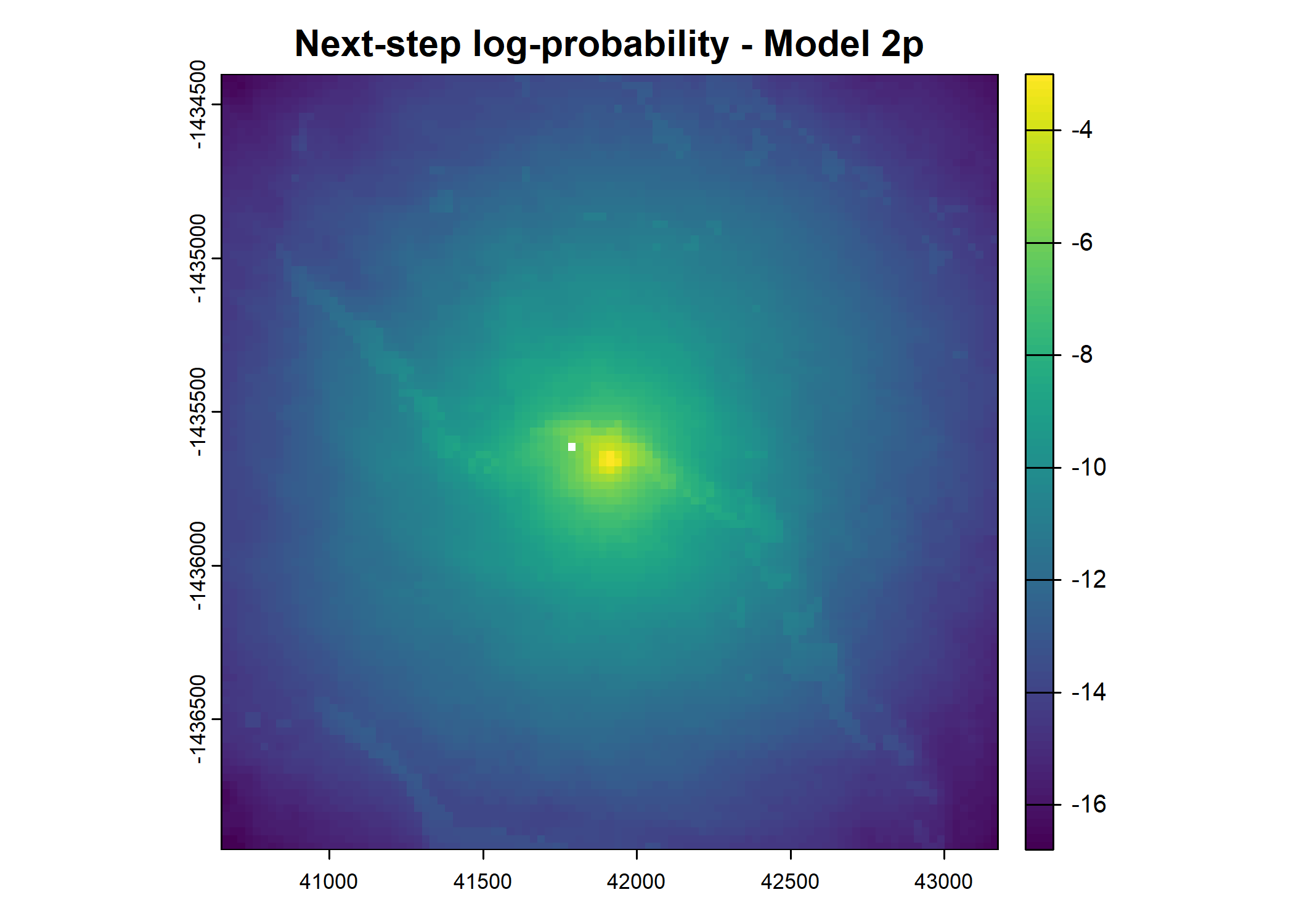

       x_       y_                   t_   id     x1_      y1_      x2_      y2_
4 41841.2 -1435635 2018-07-25T04:04:39Z 2005 41841.2 -1435635 41655.46 -1435604
    x2_cent  y2_cent                  t2_ t_diff hour_t1 yday_t1 hour_t2
4 -185.7399 31.00353 2018-07-25T05:04:27Z      1      14     206      15
  hour_t2_sin hour_t2_cos yday_t2 yday_t2_sin yday_t2_cos       sl   log_sl
4  -0.7071068  -0.7071068     206  -0.3913578  -0.9202386 188.3097 5.238088
   bearing bearing_sin bearing_cos        ta     cos_ta   x_min   x_max
4 2.976198   0.1646412  -0.9863535 -2.799767 -0.9421444 40578.7 43103.7
     y_min    y_max s2_index points_vect_cent year_t2 yday_t2_2018_base
4 -1436898 -1434373        7               NA    2018               206
  prob_habitat_ssf_0p prob_movement_ssf_0p prob_next_step_ssf_0p
4        9.907641e-05         0.0007681248           0.000797917
  prob_habitat_ssf_2p prob_movement_ssf_2p prob_next_step_ssf_2p
4                  NA                   NA                    NA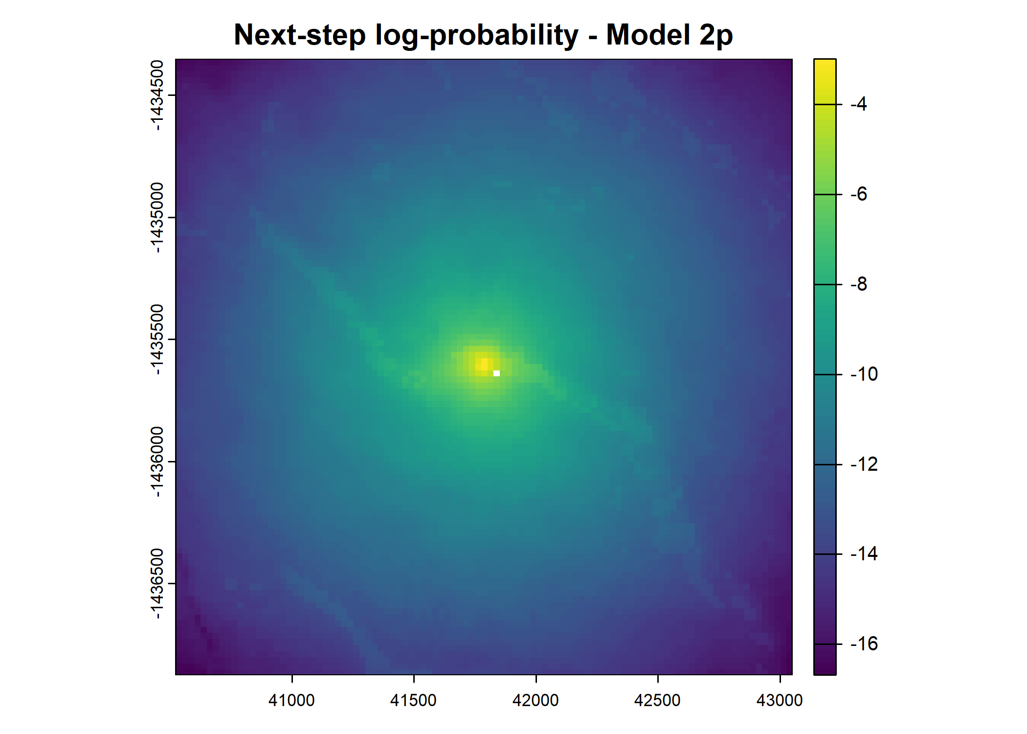
        x_       y_                   t_   id      x1_      y1_      x2_
5 41655.46 -1435604 2018-07-25T05:04:27Z 2005 41655.46 -1435604 41618.65
       y2_   x2_cent   y2_cent                  t2_ t_diff hour_t1 yday_t1
5 -1435608 -36.81141 -4.438037 2018-07-25T06:04:24Z      1      15     206
  hour_t2 hour_t2_sin hour_t2_cos yday_t2 yday_t2_sin yday_t2_cos       sl
5      16  -0.8660254        -0.5     206  -0.3913578  -0.9202386 37.07797
    log_sl  bearing bearing_sin bearing_cos        ta    cos_ta    x_min
5 3.613023 -3.02161  -0.1196947  -0.9928107 0.2853766 0.9595557 40392.96
     x_max    y_min    y_max s2_index points_vect_cent year_t2
5 42917.96 -1436867 -1434342        7               NA    2018
  yday_t2_2018_base prob_habitat_ssf_0p prob_movement_ssf_0p
5               206        9.602568e-05           0.01028661
  prob_next_step_ssf_0p prob_habitat_ssf_2p prob_movement_ssf_2p
5            0.01055869                  NA                   NA
  prob_next_step_ssf_2p
5                    NA
        x_       y_                   t_   id      x1_      y1_      x2_
6 41618.65 -1435608 2018-07-25T06:04:24Z 2005 41618.65 -1435608 41688.44
       y2_  x2_cent   y2_cent                  t2_ t_diff hour_t1 yday_t1
6 -1436126 69.78648 -517.1566 2018-07-25T07:04:28Z      1      16     206
  hour_t2 hour_t2_sin hour_t2_cos yday_t2 yday_t2_sin yday_t2_cos       sl
6      17  -0.9659258   -0.258819     206  -0.3913578  -0.9202386 521.8439
    log_sl   bearing bearing_sin bearing_cos       ta      cos_ta    x_min
6 6.257369 -1.436664  -0.9910177   0.1337306 1.584946 -0.01414957 40356.15
     x_max    y_min    y_max s2_index points_vect_cent year_t2
6 42881.15 -1436871 -1434346        7               NA    2018
  yday_t2_2018_base prob_habitat_ssf_0p prob_movement_ssf_0p
6               206        9.083069e-05         7.547135e-05
  prob_next_step_ssf_0p prob_habitat_ssf_2p prob_movement_ssf_2p
6          7.375487e-05                  NA                   NA
  prob_next_step_ssf_2p
6                    NA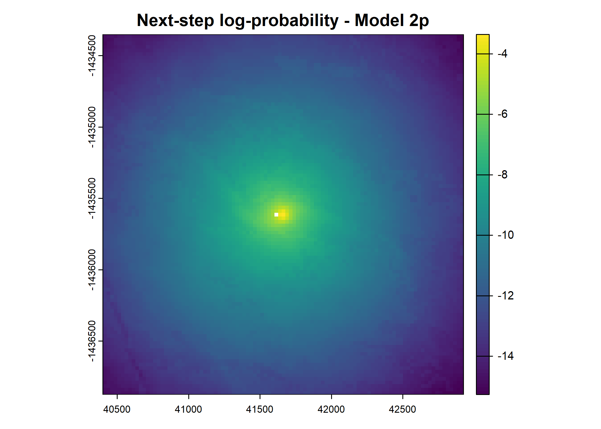

        x_       y_                   t_   id      x1_      y1_      x2_
7 41688.44 -1436126 2018-07-25T07:04:28Z 2005 41688.44 -1436126 41684.34
       y2_   x2_cent  y2_cent                  t2_ t_diff hour_t1 yday_t1
7 -1436119 -4.095906 7.020228 2018-07-25T08:04:31Z      1      17     206
  hour_t2 hour_t2_sin  hour_t2_cos yday_t2 yday_t2_sin yday_t2_cos       sl
7      18          -1 -1.83691e-16     206  -0.3913578  -0.9202386 8.127733
    log_sl  bearing bearing_sin bearing_cos        ta     cos_ta    x_min
7 2.095282 2.098953   0.8637375   -0.503942 -2.747568 -0.9233716 40425.94
     x_max    y_min    y_max s2_index points_vect_cent year_t2
7 42950.94 -1437388 -1434863        7               NA    2018
  yday_t2_2018_base prob_habitat_ssf_0p prob_movement_ssf_0p
7               206        9.167352e-05           0.02051778
  prob_next_step_ssf_0p prob_habitat_ssf_2p prob_movement_ssf_2p
7            0.01968547                  NA                   NA
  prob_next_step_ssf_2p
7                    NA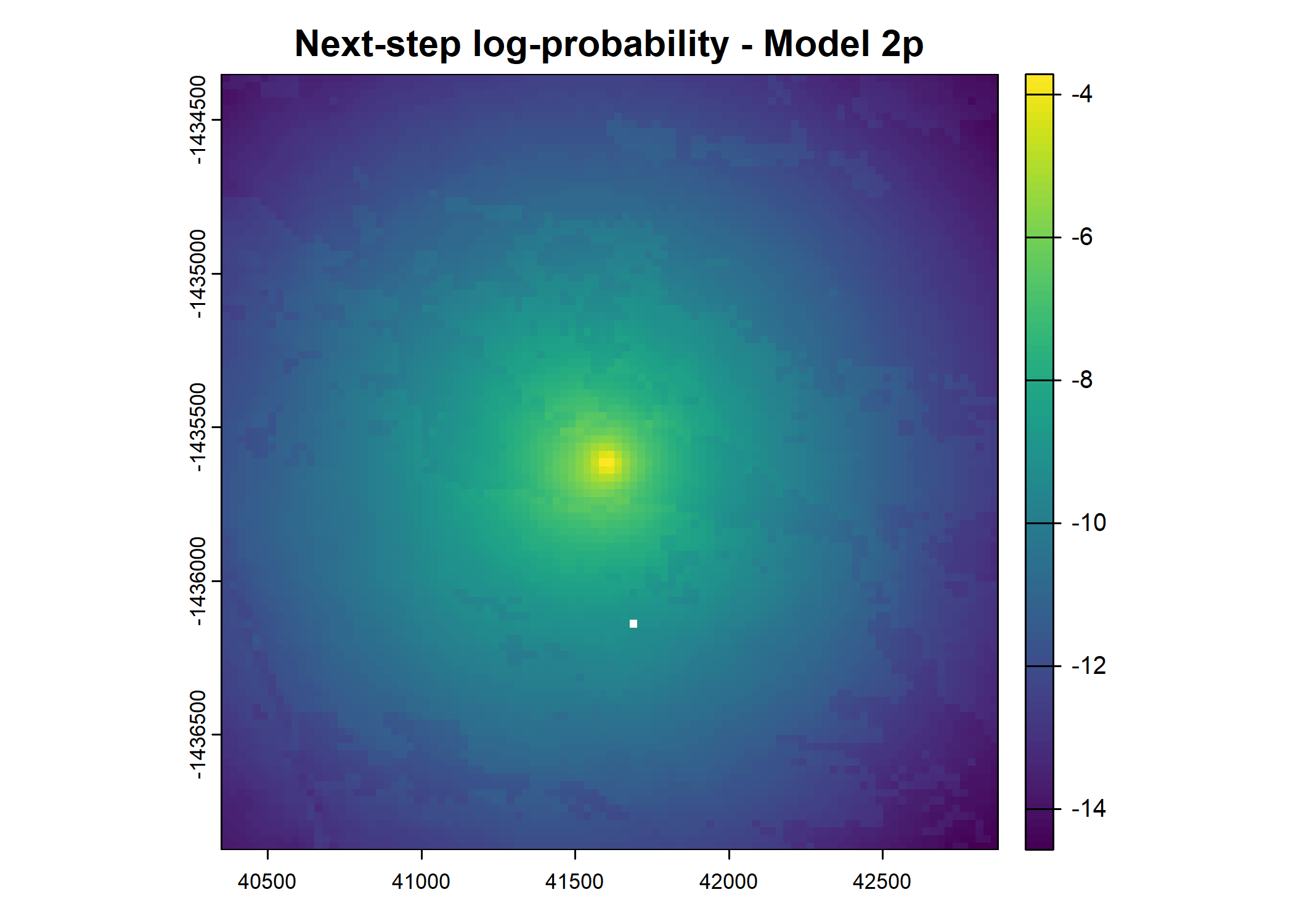
        x_       y_                   t_   id      x1_      y1_      x2_
8 41684.34 -1436119 2018-07-25T08:04:31Z 2005 41684.34 -1436119 41674.59
       y2_   x2_cent     y2_cent                  t2_ t_diff hour_t1 yday_t1
8 -1436119 -9.754289 -0.08369654 2018-07-25T09:04:33Z      1      18     206
  hour_t2 hour_t2_sin hour_t2_cos yday_t2 yday_t2_sin yday_t2_cos       sl
8      19  -0.9659258    0.258819     206  -0.3913578  -0.9202386 9.754648
    log_sl   bearing bearing_sin bearing_cos      ta    cos_ta    x_min
8 2.277744 -3.133012 -0.00858017  -0.9999632 1.05122 0.4965124 40421.84
     x_max    y_min    y_max s2_index points_vect_cent year_t2
8 42946.84 -1437381 -1434856        7               NA    2018
  yday_t2_2018_base prob_habitat_ssf_0p prob_movement_ssf_0p
8               206        9.007231e-05           0.02774303
  prob_next_step_ssf_0p prob_habitat_ssf_2p prob_movement_ssf_2p
8            0.02635727                  NA                   NA
  prob_next_step_ssf_2p
8                    NA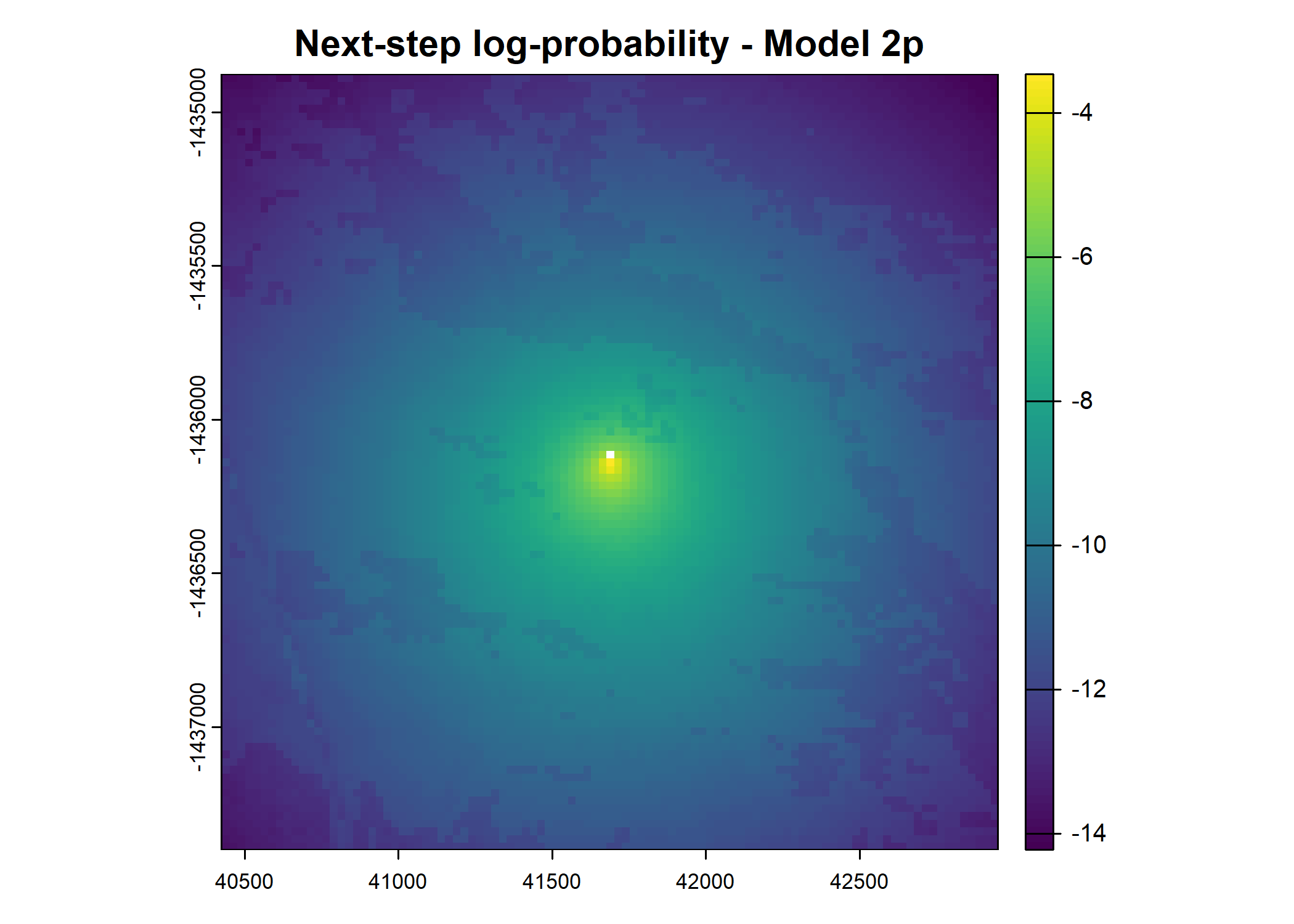
        x_       y_                   t_   id      x1_      y1_      x2_
9 41674.59 -1436119 2018-07-25T09:04:33Z 2005 41674.59 -1436119 41425.16
       y2_   x2_cent  y2_cent                  t2_ t_diff hour_t1 yday_t1
9 -1435938 -249.4296 180.3333 2018-07-25T10:04:02Z      1      19     206
  hour_t2 hour_t2_sin hour_t2_cos yday_t2 yday_t2_sin yday_t2_cos       sl
9      20  -0.8660254         0.5     206  -0.3913578  -0.9202386 307.7908
   log_sl  bearing bearing_sin bearing_cos         ta    cos_ta    x_min
9 5.72942 2.515608   0.5858955  -0.8103866 -0.6345649 0.8053297 40412.09
     x_max    y_min    y_max s2_index points_vect_cent year_t2
9 42937.09 -1437381 -1434856        7               NA    2018
  yday_t2_2018_base prob_habitat_ssf_0p prob_movement_ssf_0p
9               206        9.566552e-05         0.0004125345
  prob_next_step_ssf_0p prob_habitat_ssf_2p prob_movement_ssf_2p
9          0.0004177971                  NA                   NA
  prob_next_step_ssf_2p
9                    NA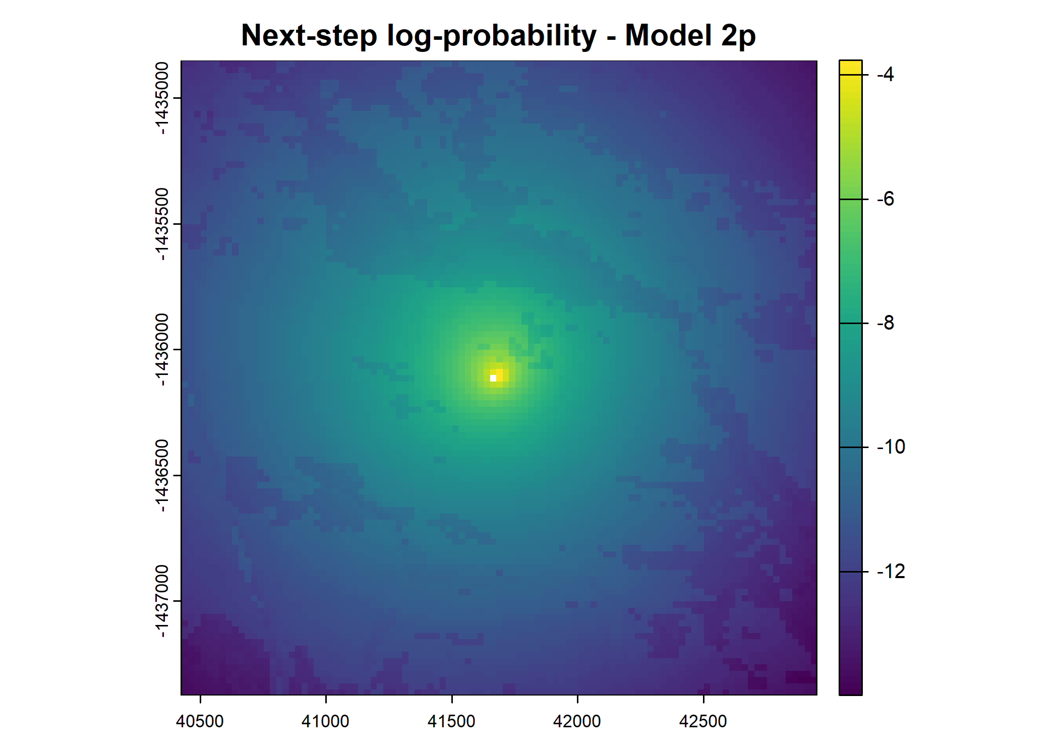
         x_       y_                   t_   id      x1_      y1_      x2_
10 41425.16 -1435938 2018-07-25T10:04:02Z 2005 41425.16 -1435938 40563.21
        y2_   x2_cent  y2_cent                  t2_ t_diff hour_t1 yday_t1
10 -1435841 -861.9445 97.45269 2018-07-25T11:04:04Z      1      20     206
   hour_t2 hour_t2_sin hour_t2_cos yday_t2 yday_t2_sin yday_t2_cos       sl
10      21  -0.7071068   0.7071068     206  -0.3913578  -0.9202386 867.4361
     log_sl  bearing bearing_sin bearing_cos        ta    cos_ta    x_min
10 6.765542 3.029009   0.1123457  -0.9936692 0.5134012 0.8710791 40162.66
      x_max    y_min    y_max s2_index points_vect_cent year_t2
10 42687.66 -1437201 -1434676        7               NA    2018
   yday_t2_2018_base prob_habitat_ssf_0p prob_movement_ssf_0p
10               206         0.000109441          1.74964e-05
   prob_next_step_ssf_0p prob_habitat_ssf_2p prob_movement_ssf_2p
10          2.029205e-05                  NA                   NA
   prob_next_step_ssf_2p
10                    NA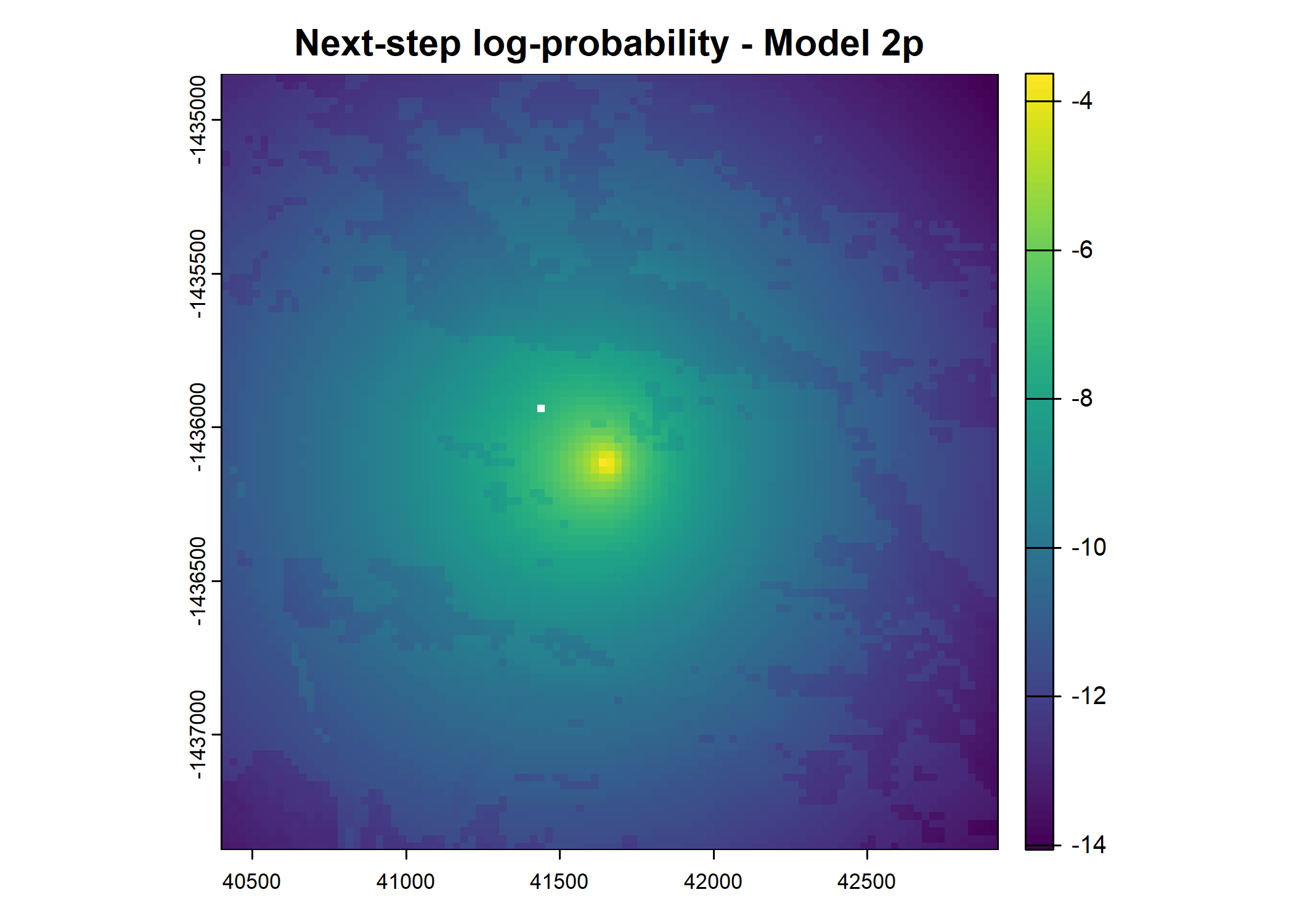

         x_       y_                   t_   id      x1_      y1_      x2_
11 40563.21 -1435841 2018-07-25T11:04:04Z 2005 40563.21 -1435841 40512.76
        y2_   x2_cent  y2_cent                  t2_ t_diff hour_t1 yday_t1
11 -1435777 -50.44988 63.87376 2018-07-25T12:05:13Z      1      21     206
   hour_t2 hour_t2_sin hour_t2_cos yday_t2 yday_t2_sin yday_t2_cos       sl
11      22        -0.5   0.8660254     206  -0.3913578  -0.9202386 81.39439
     log_sl bearing bearing_sin bearing_cos         ta    cos_ta    x_min
11 4.399306 2.23931    0.784744    -0.61982 -0.7896996 0.7040587 39300.71
      x_max    y_min    y_max s2_index points_vect_cent year_t2
11 41825.71 -1437103 -1434578        7               NA    2018
   yday_t2_2018_base prob_habitat_ssf_0p prob_movement_ssf_0p
11               206        0.0001102691          0.005606582
   prob_next_step_ssf_0p prob_habitat_ssf_2p prob_movement_ssf_2p
11           0.005993663                  NA                   NA
   prob_next_step_ssf_2p
11                    NA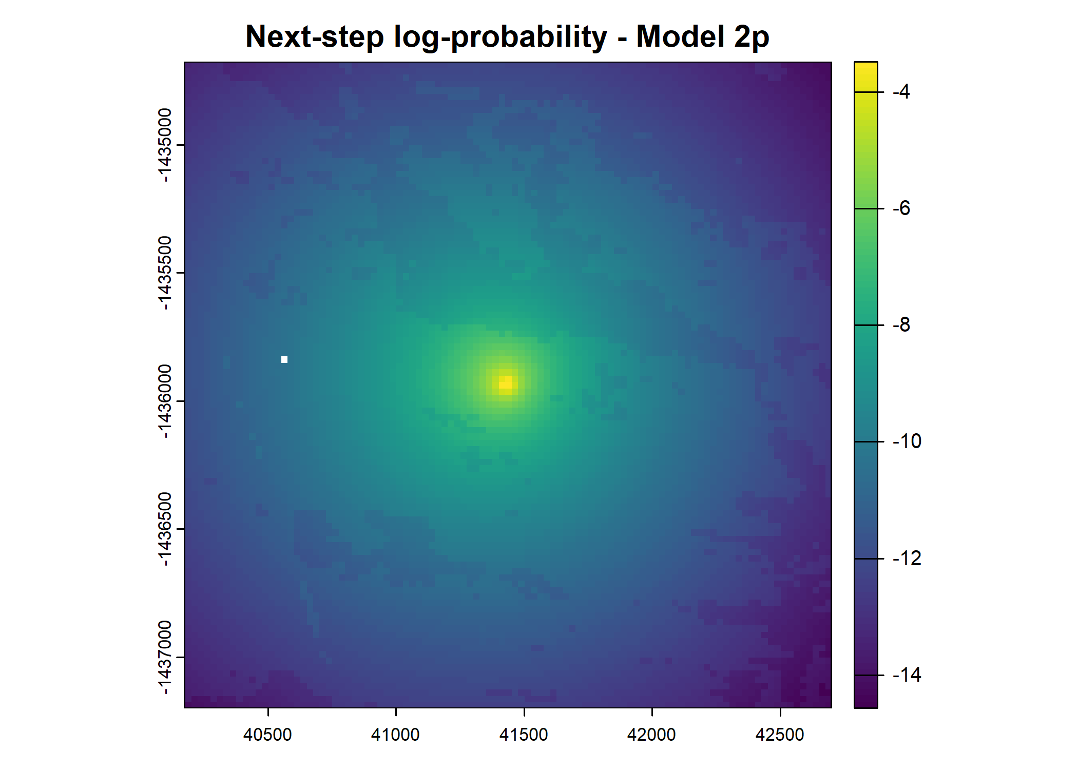

37.79 sec elapsed83.45 sec elapsedCode
test_data_correction <- test_data %>% drop_na(prob_habitat_ssf_0p) %>%
  select(t_,
         prob_habitat_ssf_0p, prob_habitat_ssf_2p,
         prob_movement_ssf_0p, prob_movement_ssf_2p,
         prob_next_step_ssf_0p, prob_next_step_ssf_2p
         ) %>%
  mutate(t_ = lubridate::as_datetime(t_)) %>%
  pivot_longer(cols = !c(t_),
             names_to = "model", values_to = "prob")

ggplot() +
  geom_hline(yintercept = 0.000098, linetype = "dashed") +
  geom_line(data=test_data_correction %>% filter(),
            aes(x = t_, y = prob, colour = model)) +
  theme_bw()
Warning: Removed 4 rows containing missing values or values outside the scale range
(`geom_line()`).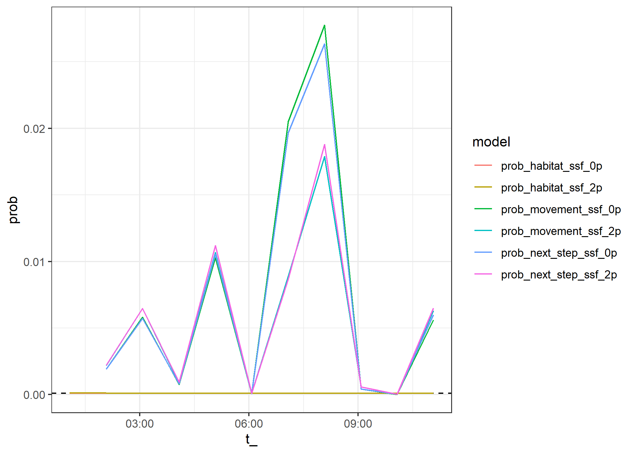
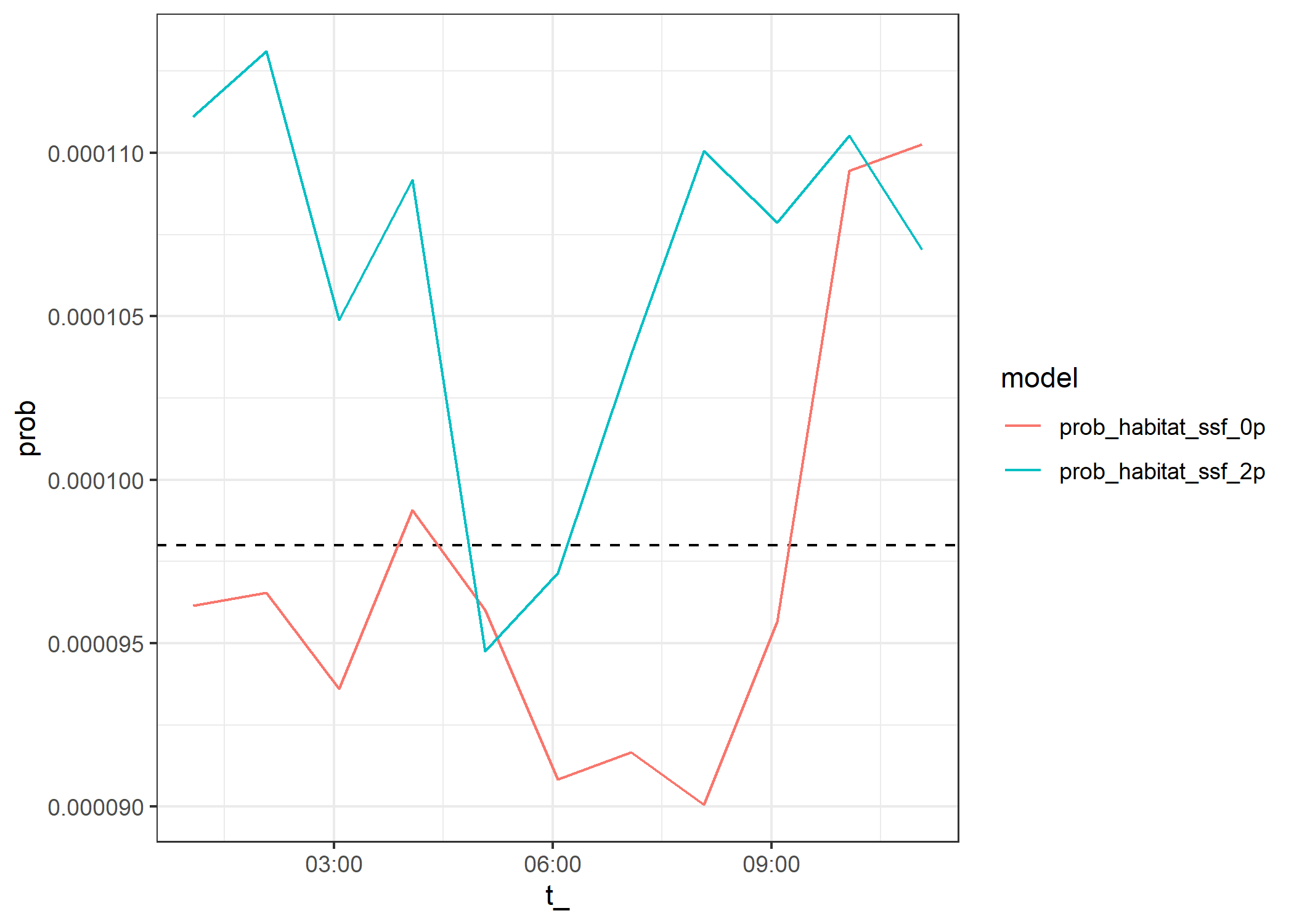
Code
test_data_correction <- test_data %>% drop_na(prob_habitat_ssf_0p) %>%
  select(t_,
         prob_habitat_ssf_0p, prob_habitat_ssf_2p
         # prob_movement_ssf_0p, prob_movement_ssf_2p,
         # prob_next_step_ssf_0p, prob_next_step_ssf_2p
         ) %>%
  mutate(t_ = lubridate::as_datetime(t_)) %>%
  pivot_longer(cols = !c(t_),
             names_to = "model", values_to = "prob")

ggplot() +
  geom_hline(yintercept = 0.000098, linetype = "dashed") +
  geom_line(data=test_data_correction %>% filter(),
            aes(x = t_, y = prob, colour = model)) +
  theme_bw()