SSF Model Fitting

To compare the next-step predictions of the deepSSF models to SSF models, we need to fit some SSF models to the same data and covariates. Here we fit SSF models with and without temporal harmonics to buffalo data, which is similar to the approach in Forrest et al. (2024) except that here we are just fitting the models to the focal individual, rather than to multiple individuals.
We use the estimated parameters of the SSF models to generate next-step predictions of the SSF models in the SSF Validation script, and compare these to the next-step predictions of the deepSSF models.
Whilst we have included temporal dynamics on an daily time-scale using the harmonics, also including seasonal temporal dynamics (such that daily behaviours also change across seasons - requiring an interaction between the daily and seasonal harmonics) is difficult. We have therefore only fitted the SSF models with daily temporal dynamics.
We have also not fitted the SSF models to the Sentinel-2 data, as we have done with the deepSSF models.
Load packages
Importing buffalo data
Import the buffalo data with random steps and extracted covariates that we created for the paper Forrest et al. (2024), in the script Ecography_DynamicSSF_1_Step_generation. This repo can be found at: swforrest/dynamic_SSF_sims.
Here we create the sine and cosine terms that were interact with each of the covariates to fit temporally varying parameters.
Importing data
Rows: 1165406 Columns: 22
── Column specification ────────────────────────────────────────────────────────
Delimiter: ","
dbl  (18): id, burst_, x1_, x2_, y1_, y2_, sl_, ta_, dt_, hour_t2, step_id_,...
lgl   (1): case_
dttm  (3): t1_, t2_, t2_rounded

ℹ Use `spec()` to retrieve the full column specification for this data.
ℹ Specify the column types or set `show_col_types = FALSE` to quiet this message.
Importing data
buffalo_data_all <- buffalo_data_all %>%
  mutate(t1_ = lubridate::with_tz(buffalo_data_all$t1_, tzone = "Australia/Darwin"),
         t2_ = lubridate::with_tz(buffalo_data_all$t2_, tzone = "Australia/Darwin"))

buffalo_data_all <- buffalo_data_all %>%
  mutate(id_num = as.numeric(factor(id)),
         step_id = step_id_,
         x1 = x1_, x2 = x2_,
         y1 = y1_, y2 = y2_,
         t1 = t1_,
         t1_rounded = round_date(buffalo_data_all$t1_, "hour"),
         hour_t1 = hour(t1_rounded),
         t2 = t2_,
         t2_rounded = round_date(buffalo_data_all$t2_, "hour"),
         hour_t2 = hour(t2_rounded),
         hour = hour_t2,
         yday = yday(t1_),
         year = year(t1_),
         month = month(t1_),
         sl = sl_,
         log_sl = log(sl_),
         ta = ta_,
         cos_ta = cos(ta_),
         # scale canopy cover from 0 to 1
         canopy_01 = canopy_cover/100,
         # here we create the harmonic terms for the hour of the day
         # for seasonal effects, change hour to yday (which is tau in the manuscript),
         # and 24 to 365 (which is T)
         hour_s1 = sin(2*pi*hour/24),
         hour_s2 = sin(4*pi*hour/24),
         hour_s3 = sin(6*pi*hour/24),
         hour_c1 = cos(2*pi*hour/24),
         hour_c2 = cos(4*pi*hour/24),
         hour_c3 = cos(6*pi*hour/24))

# to select a single year of data
# buffalo_data_all <- buffalo_data_all %>% filter(t1 < "2019-07-25 09:32:42 ACST")

buffalo_ids <- unique(buffalo_data_all$id)

# Timeline of buffalo data
buffalo_data_all %>% ggplot(aes(x = t1, y = factor(id), colour = factor(id))) +
  geom_point(alpha = 0.1) +
  scale_y_discrete("Buffalo ID") +
  scale_x_datetime("Date") +
  scale_colour_viridis_d() +
  theme_bw() +
  theme(legend.position = "none")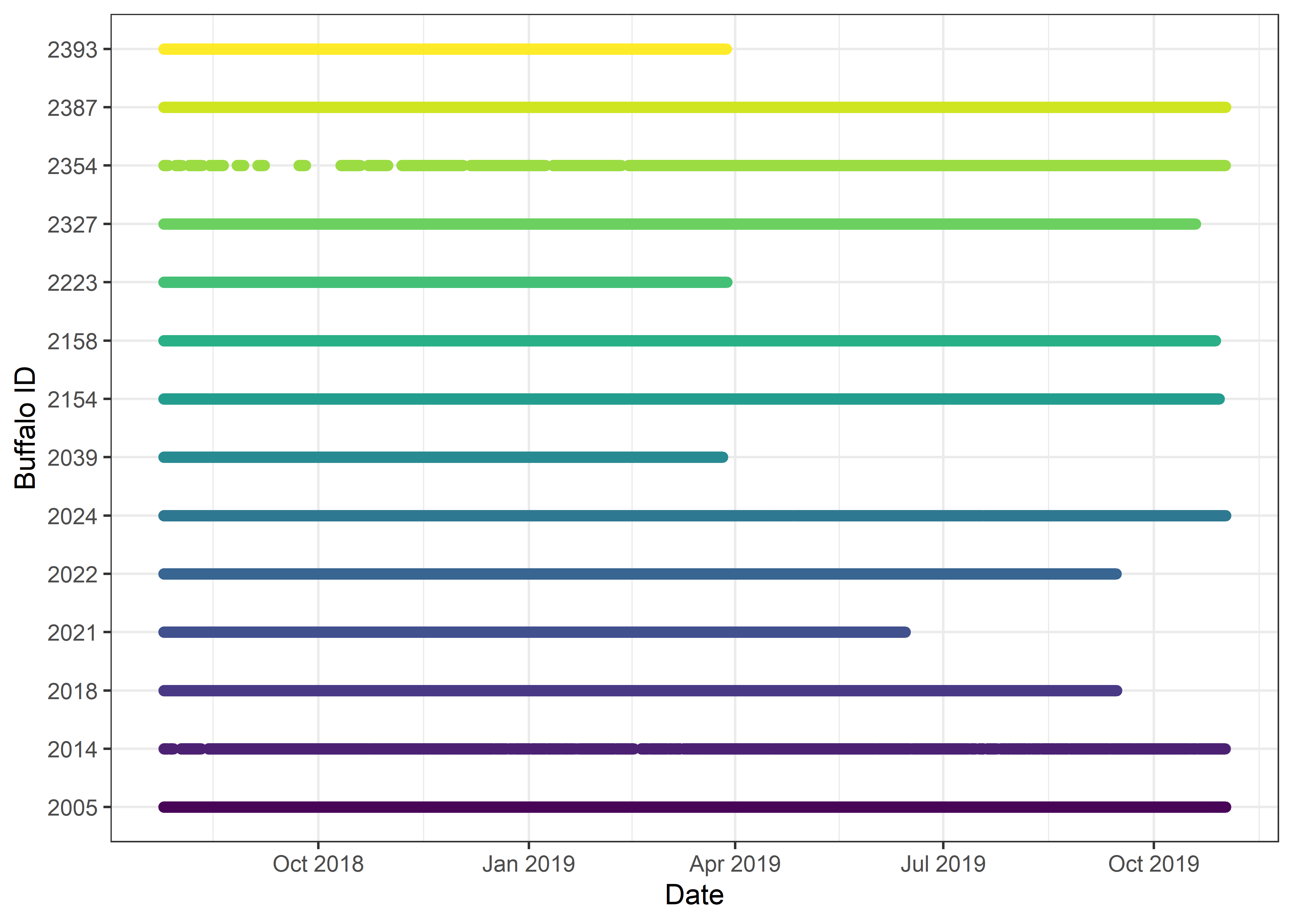
Fitting the models
Creating a data matrix
First we create a data matrix to be provided to the model, and then we scale and centre the full data matrix, with respect to each of the columns. That means that all variables are scaled and centred after the data has been split into wet and dry season data, and also after creating the quadratic and harmonic terms (when using them).
We should only include covariates in the data matrix that will be used in the model formula.
Models
- 0p = 0 pairs of harmonics
- 1p = 1 pair of harmonics
- 2p = 2 pairs of harmonics
- 3p = 3 pairs of harmonics
For the dynamic models, we start to add the harmonic terms. As we have already created the harmonic terms for the hour of the day (s1, c1, s2, etc), we just interact (multiply) these with each of the covariates, including the quadratic terms, prior to model fitting. We store the scaling and centering variables to reconstruct the natural scale coefficients.
To provide some intuition about harmonic regression we have created a walkthrough script for Forrest et al. (2024), in the script Ecography_DynamicSSF_Walkthrough_Harmonics_and_selection_surfaces, which can be found at: swforrest/dynamic_SSF_sims, that introduces harmonics and how they can be used to model temporal variation in the data. It will help provide some understand the model outputs and how we construct the temporally varying coefficients in this script.
Selecting data
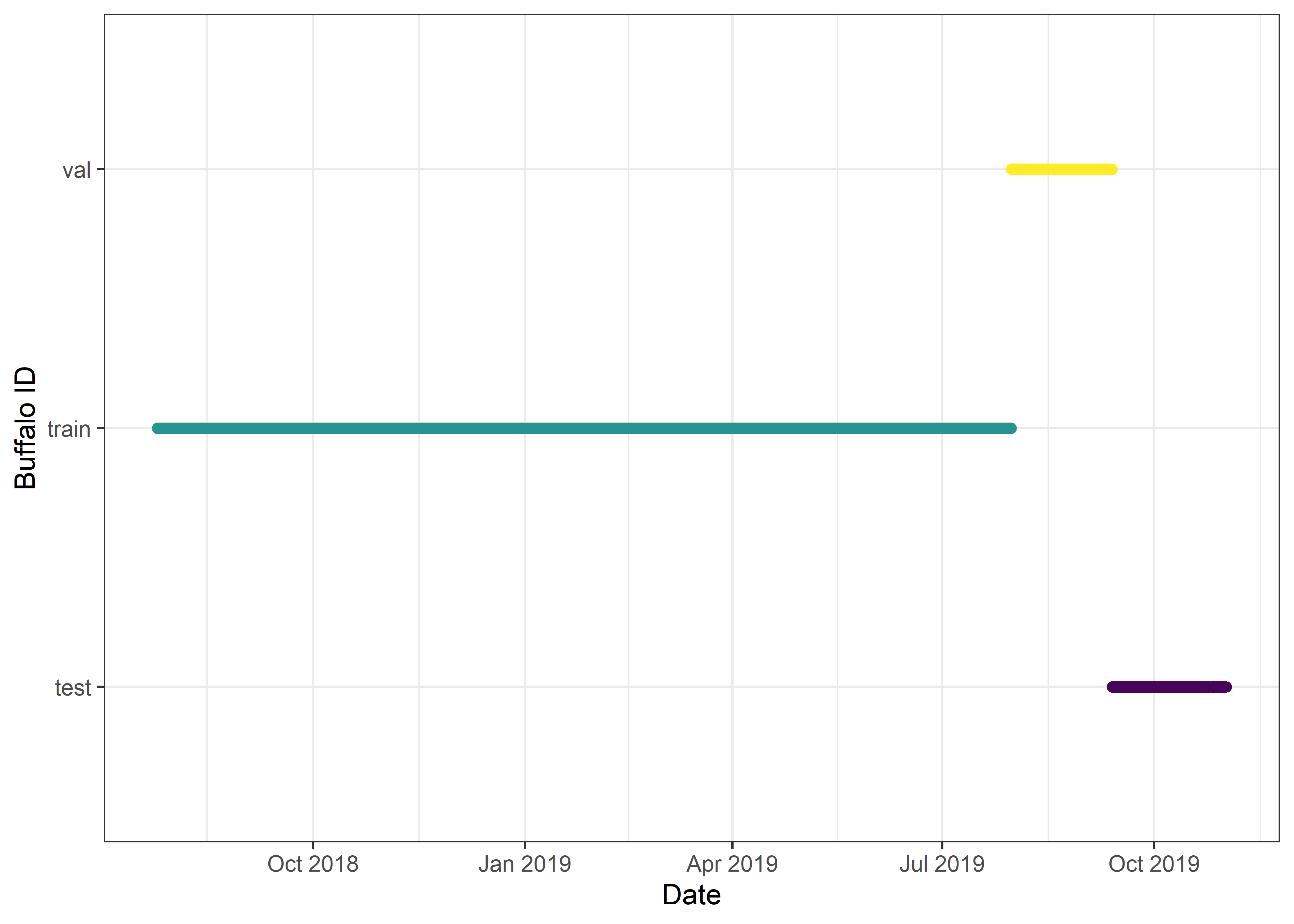
Split the data into train/validate/test
This is to match the splitting of data that was used to train/fit the deepSSF model. There we used an 80/10/10 split, with 80% of the data for training, 10% for validation, and 10% for testing.
We will follow that same split here, although the validation set is specific to deep learning (it is used to assess when to reduce the learning rate and stop training), with the 10% test data to be used for the held-out validation dataset.
Code
training_split <- 0.8 # 80% of the data will be used for fitting the model
validation_split <- 0.1 # 10% of the data will be used for validation (which isn't used here)
test_split <- 0.1 # 10% of the data will be used for testing (model evaluation)

# Calculate the number of samples for each split
n_samples <- nrow(buffalo_id)

n_train <- floor(training_split * n_samples)
n_val <- floor(validation_split * n_samples)
n_test <- n_samples - n_train - n_val  # Ensure they sum to total number of samples

# Get the start and end indices for each split
train_end <- floor(training_split * n_samples)
val_end <- floor((training_split + validation_split) * n_samples)

# Generate indices for each split
train_indices <- 1:train_end
val_indices <- (train_end + 1):val_end
test_indices <- (val_end + 1):n_samples

# Create a new column in the data frame to indicate the dataset
buffalo_id <- buffalo_id %>% mutate(dataset = NA)

# Add which type of dataset the location should be assigned to
buffalo_id$dataset[train_indices] <- "train"
buffalo_id$dataset[val_indices] <- "val"
buffalo_id$dataset[test_indices] <- "test"

# Split the dataset sequentially
buffalo_data <- buffalo_id[train_indices, ]
buffalo_data_val <- buffalo_id[val_indices, ]
buffalo_data_test <- buffalo_id[test_indices, ]

# Print the number of samples in each split
cat("Number of training samples:   ", nrow(buffalo_data), "\n")
Number of training samples: 85852 Number of validation samples: 10732 Number of testing samples: 10732 Code
From Pytorch
There is some loss of samples due to them being larger than the spatial extent, and of course there are no randomly sampled locations
- Number of training samples: 8082
- Number of validation samples: 1010
- Number of testing samples: 1011
Code
buffalo_data_matrix_unscaled <- buffalo_data %>% transmute(

  ndvi = ndvi_temporal,
  ndvi_sq = ndvi_temporal ^ 2,
  canopy = canopy_01,
  canopy_sq = canopy_01 ^ 2,
  slope = slope,
  herby = veg_herby,
  step_l = sl,
  log_step_l = log_sl,
  cos_turn_a = cos_ta)

buffalo_data_matrix_scaled <- scale(buffalo_data_matrix_unscaled)

# save the scaling values to recover the natural scale of the coefficients
# which is required for the simulations
# (so then environmental variables don't need to be scaled)
mean_vals <- attr(buffalo_data_matrix_scaled, "scaled:center")
sd_vals <- attr(buffalo_data_matrix_scaled, "scaled:scale")
scaling_attributes_0p <- data.frame(variable = names(buffalo_data_matrix_unscaled),
                                    mean = mean_vals, sd = sd_vals)

# add the id, step_id columns and presence/absence columns to
# the scaled data matrix for model fitting
buffalo_data_scaled_0p <- data.frame(id = buffalo_data$id,
                                     step_id = buffalo_data$step_id,
                                     y = buffalo_data$y,
                                     buffalo_data_matrix_scaled)
Code
buffalo_data_matrix_unscaled <- buffalo_data %>% transmute(

  # the 'linear' term
  ndvi = ndvi_temporal,
  # interact with the harmonic terms
  ndvi_s1 = ndvi_temporal * hour_s1,
  ndvi_c1 = ndvi_temporal * hour_c1,

  ndvi_sq = ndvi_temporal ^ 2,
  ndvi_sq_s1 = (ndvi_temporal ^ 2) * hour_s1,
  ndvi_sq_c1 = (ndvi_temporal ^ 2) * hour_c1,

  canopy = canopy_01,
  canopy_s1 = canopy_01 * hour_s1,
  canopy_c1 = canopy_01 * hour_c1,

  canopy_sq = canopy_01 ^ 2,
  canopy_sq_s1 = (canopy_01 ^ 2) * hour_s1,
  canopy_sq_c1 = (canopy_01 ^ 2) * hour_c1,

  slope = slope,
  slope_s1 = slope * hour_s1,
  slope_c1 = slope * hour_c1,

  herby = veg_herby,
  herby_s1 = veg_herby * hour_s1,
  herby_c1 = veg_herby * hour_c1,

  step_l = sl,
  step_l_s1 = sl * hour_s1,
  step_l_c1 = sl * hour_c1,

  log_step_l = log_sl,
  log_step_l_s1 = log_sl * hour_s1,
  log_step_l_c1 = log_sl * hour_c1,

  cos_turn_a = cos_ta,
  cos_turn_a_s1 = cos_ta * hour_s1,
  cos_turn_a_c1 = cos_ta * hour_c1)

buffalo_data_matrix_scaled <- scale(buffalo_data_matrix_unscaled)

mean_vals <- attr(buffalo_data_matrix_scaled, "scaled:center")
sd_vals <- attr(buffalo_data_matrix_scaled, "scaled:scale")
scaling_attributes_1p <- data.frame(variable = names(buffalo_data_matrix_unscaled),
                                    mean = mean_vals, sd = sd_vals)

buffalo_data_scaled_1p <- data.frame(id = buffalo_data$id,
                                     step_id = buffalo_data$step_id,
                                     y = buffalo_data$y,
                                     buffalo_data_matrix_scaled)
Code
buffalo_data_matrix_unscaled <- buffalo_data %>% transmute(

  ndvi = ndvi_temporal,
  ndvi_s1 = ndvi_temporal * hour_s1,
  ndvi_s2 = ndvi_temporal * hour_s2,
  ndvi_c1 = ndvi_temporal * hour_c1,
  ndvi_c2 = ndvi_temporal * hour_c2,

  ndvi_sq = ndvi_temporal ^ 2,
  ndvi_sq_s1 = (ndvi_temporal ^ 2) * hour_s1,
  ndvi_sq_s2 = (ndvi_temporal ^ 2) * hour_s2,
  ndvi_sq_c1 = (ndvi_temporal ^ 2) * hour_c1,
  ndvi_sq_c2 = (ndvi_temporal ^ 2) * hour_c2,

  canopy = canopy_01,
  canopy_s1 = canopy_01 * hour_s1,
  canopy_s2 = canopy_01 * hour_s2,
  canopy_c1 = canopy_01 * hour_c1,
  canopy_c2 = canopy_01 * hour_c2,

  canopy_sq = canopy_01 ^ 2,
  canopy_sq_s1 = (canopy_01 ^ 2) * hour_s1,
  canopy_sq_s2 = (canopy_01 ^ 2) * hour_s2,
  canopy_sq_c1 = (canopy_01 ^ 2) * hour_c1,
  canopy_sq_c2 = (canopy_01 ^ 2) * hour_c2,

  slope = slope,
  slope_s1 = slope * hour_s1,
  slope_s2 = slope * hour_s2,
  slope_c1 = slope * hour_c1,
  slope_c2 = slope * hour_c2,

  herby = veg_herby,
  herby_s1 = veg_herby * hour_s1,
  herby_s2 = veg_herby * hour_s2,
  herby_c1 = veg_herby * hour_c1,
  herby_c2 = veg_herby * hour_c2,

  step_l = sl,
  step_l_s1 = sl * hour_s1,
  step_l_s2 = sl * hour_s2,
  step_l_c1 = sl * hour_c1,
  step_l_c2 = sl * hour_c2,

  log_step_l = log_sl,
  log_step_l_s1 = log_sl * hour_s1,
  log_step_l_s2 = log_sl * hour_s2,
  log_step_l_c1 = log_sl * hour_c1,
  log_step_l_c2 = log_sl * hour_c2,

  cos_turn_a = cos_ta,
  cos_turn_a_s1 = cos_ta * hour_s1,
  cos_turn_a_s2 = cos_ta * hour_s2,
  cos_turn_a_c1 = cos_ta * hour_c1,
  cos_turn_a_c2 = cos_ta * hour_c2)

buffalo_data_matrix_scaled <- scale(buffalo_data_matrix_unscaled)

mean_vals <- attr(buffalo_data_matrix_scaled, "scaled:center")
sd_vals <- attr(buffalo_data_matrix_scaled, "scaled:scale")
scaling_attributes_2p <- data.frame(variable = names(buffalo_data_matrix_unscaled),
                                    mean = mean_vals, sd = sd_vals)

buffalo_data_scaled_2p <- data.frame(id = buffalo_data$id,
                                     step_id = buffalo_data$step_id,
                                     y = buffalo_data$y,
                                     buffalo_data_matrix_scaled)
Code
buffalo_data_matrix_unscaled <- buffalo_data %>% transmute(

  ndvi = ndvi_temporal,
  ndvi_s1 = ndvi_temporal * hour_s1,
  ndvi_s2 = ndvi_temporal * hour_s2,
  ndvi_s3 = ndvi_temporal * hour_s3,
  ndvi_c1 = ndvi_temporal * hour_c1,
  ndvi_c2 = ndvi_temporal * hour_c2,
  ndvi_c3 = ndvi_temporal * hour_c3,

  ndvi_sq = ndvi_temporal ^ 2,
  ndvi_sq_s1 = (ndvi_temporal ^ 2) * hour_s1,
  ndvi_sq_s2 = (ndvi_temporal ^ 2) * hour_s2,
  ndvi_sq_s3 = (ndvi_temporal ^ 2) * hour_s3,
  ndvi_sq_c1 = (ndvi_temporal ^ 2) * hour_c1,
  ndvi_sq_c2 = (ndvi_temporal ^ 2) * hour_c2,
  ndvi_sq_c3 = (ndvi_temporal ^ 2) * hour_c3,

  canopy = canopy_01,
  canopy_s1 = canopy_01 * hour_s1,
  canopy_s2 = canopy_01 * hour_s2,
  canopy_s3 = canopy_01 * hour_s3,
  canopy_c1 = canopy_01 * hour_c1,
  canopy_c2 = canopy_01 * hour_c2,
  canopy_c3 = canopy_01 * hour_c3,

  canopy_sq = canopy_01 ^ 2,
  canopy_sq_s1 = (canopy_01 ^ 2) * hour_s1,
  canopy_sq_s2 = (canopy_01 ^ 2) * hour_s2,
  canopy_sq_s3 = (canopy_01 ^ 2) * hour_s3,
  canopy_sq_c1 = (canopy_01 ^ 2) * hour_c1,
  canopy_sq_c2 = (canopy_01 ^ 2) * hour_c2,
  canopy_sq_c3 = (canopy_01 ^ 2) * hour_c3,

  slope = slope,
  slope_s1 = slope * hour_s1,
  slope_s2 = slope * hour_s2,
  slope_s3 = slope * hour_s3,
  slope_c1 = slope * hour_c1,
  slope_c2 = slope * hour_c2,
  slope_c3 = slope * hour_c3,

  herby = veg_herby,
  herby_s1 = veg_herby * hour_s1,
  herby_s2 = veg_herby * hour_s2,
  herby_s3 = veg_herby * hour_s3,
  herby_c1 = veg_herby * hour_c1,
  herby_c2 = veg_herby * hour_c2,
  herby_c3 = veg_herby * hour_c3,

  step_l = sl,
  step_l_s1 = sl * hour_s1,
  step_l_s2 = sl * hour_s2,
  step_l_s3 = sl * hour_s3,
  step_l_c1 = sl * hour_c1,
  step_l_c2 = sl * hour_c2,
  step_l_c3 = sl * hour_c3,

  log_step_l = log_sl,
  log_step_l_s1 = log_sl * hour_s1,
  log_step_l_s2 = log_sl * hour_s2,
  log_step_l_s3 = log_sl * hour_s3,
  log_step_l_c1 = log_sl * hour_c1,
  log_step_l_c2 = log_sl * hour_c2,
  log_step_l_c3 = log_sl * hour_c3,

  cos_turn_a = cos_ta,
  cos_turn_a_s1 = cos_ta * hour_s1,
  cos_turn_a_s2 = cos_ta * hour_s2,
  cos_turn_a_s3 = cos_ta * hour_s3,
  cos_turn_a_c1 = cos_ta * hour_c1,
  cos_turn_a_c2 = cos_ta * hour_c2,
  cos_turn_a_c3 = cos_ta * hour_c3)

buffalo_data_matrix_scaled <- scale(buffalo_data_matrix_unscaled)

mean_vals <- attr(buffalo_data_matrix_scaled, "scaled:center")
sd_vals <- attr(buffalo_data_matrix_scaled, "scaled:scale")
scaling_attributes_3p <- data.frame(variable = names(buffalo_data_matrix_unscaled),
                                    mean = mean_vals, sd = sd_vals)

buffalo_data_scaled_3p <- data.frame(id = buffalo_data$id,
                                     step_id = buffalo_data$step_id,
                                     y = buffalo_data$y,
                                     buffalo_data_matrix_scaled)
Model formula
As we have already precomputed and scaled the covariates, quadratic terms and interactions with the harmonics, we just include each parameter as a linear predictor.
Code
formula_1p <- y ~

  ndvi +
  ndvi_s1 +
  ndvi_c1 +

  ndvi_sq +
  ndvi_sq_s1 +
  ndvi_sq_c1 +

  canopy +
  canopy_s1 +
  canopy_c1 +

  canopy_sq +
  canopy_sq_s1 +
  canopy_sq_c1 +

  slope +
  slope_s1 +
  slope_c1 +

  herby +
  herby_s1 +
  herby_c1 +

  step_l +
  step_l_s1 +
  step_l_c1 +

  log_step_l +
  log_step_l_s1 +
  log_step_l_c1 +

  cos_turn_a +
  cos_turn_a_s1 +
  cos_turn_a_c1 +

  strata(step_id)
Code
formula_2p <- y ~

  ndvi +
  ndvi_s1 +
  ndvi_s2 +
  ndvi_c1 +
  ndvi_c2 +

  ndvi_sq +
  ndvi_sq_s1 +
  ndvi_sq_s2 +
  ndvi_sq_c1 +
  ndvi_sq_c2 +

  canopy +
  canopy_s1 +
  canopy_s2 +
  canopy_c1 +
  canopy_c2 +

  canopy_sq +
  canopy_sq_s1 +
  canopy_sq_s2 +
  canopy_sq_c1 +
  canopy_sq_c2 +

  slope +
  slope_s1 +
  slope_s2 +
  slope_c1 +
  slope_c2 +

  herby +
  herby_s1 +
  herby_s2 +
  herby_c1 +
  herby_c2 +

  step_l +
  step_l_s1 +
  step_l_s2 +
  step_l_c1 +
  step_l_c2 +

  log_step_l +
  log_step_l_s1 +
  log_step_l_s2 +
  log_step_l_c1 +
  log_step_l_c2 +

  cos_turn_a +
  cos_turn_a_s1 +
  cos_turn_a_s2 +
  cos_turn_a_c1 +
  cos_turn_a_c2 +

  strata(step_id)
Code
formula_3p <- y ~

  ndvi +
  ndvi_s1 +
  ndvi_s2 +
  ndvi_s3 +
  ndvi_c1 +
  ndvi_c2 +
  ndvi_c3 +

  ndvi_sq +
  ndvi_sq_s1 +
  ndvi_sq_s2 +
  ndvi_sq_s3 +
  ndvi_sq_c1 +
  ndvi_sq_c2 +
  ndvi_sq_c3 +

  canopy +
  canopy_s1 +
  canopy_s2 +
  canopy_s3 +
  canopy_c1 +
  canopy_c2 +
  canopy_c3 +

  canopy_sq +
  canopy_sq_s1 +
  canopy_sq_s2 +
  canopy_sq_s3 +
  canopy_sq_c1 +
  canopy_sq_c2 +
  canopy_sq_c3 +

  slope +
  slope_s1 +
  slope_s2 +
  slope_s3 +
  slope_c1 +
  slope_c2 +
  slope_c3 +

  herby +
  herby_s1 +
  herby_s2 +
  herby_s3 +
  herby_c1 +
  herby_c2 +
  herby_c3 +

  step_l +
  step_l_s1 +
  step_l_s2 +
  step_l_s3 +
  step_l_c1 +
  step_l_c2 +
  step_l_c3 +

  log_step_l +
  log_step_l_s1 +
  log_step_l_s2 +
  log_step_l_s3 +
  log_step_l_c1 +
  log_step_l_c2 +
  log_step_l_c3 +

  cos_turn_a +
  cos_turn_a_s1 +
  cos_turn_a_s2 +
  cos_turn_a_s3 +
  cos_turn_a_c1 +
  cos_turn_a_c2 +
  cos_turn_a_c3 +

  strata(step_id)
Fit the model
As we have already fitted the model, we will load it here, but if the model_fit file doesn’t exist, it will run the model fitting code. Be careful here that if you change the model formula, you will need to delete or rename the model_fit file to re-run the model fitting code, otherwise it will just load the previous model.
We are fitting a single model to the focal individual.
Code
if(file.exists(paste0("ssf_coefficients/model_id", focal_id, "_0p_harms_80-10-10.rds"))) {

  model_0p_harms <- readRDS(paste0("ssf_coefficients/model_id", focal_id, "_0p_harms_80-10-10.rds"))
  print("Read existing model")

} else {

  tic()
    model_0p_harms <- fit_clogit(formula = formula_0p,
                                 data = buffalo_data_scaled_0p)
  toc()

  # save model object
  saveRDS(model_0p_harms, file = paste0("ssf_coefficients/model_id", focal_id, "_0p_harms_80-10-10.rds"))

  print("Fitted model")
  beep(sound = 2)

}
[1] "Read existing model"$model
Call:
survival::clogit(formula, data = data, ...)
coef exp(coef) se(coef) z p
ndvi 0.185889 1.204288 0.058928 3.155 0.00161
ndvi_sq -0.069088 0.933245 0.061755 -1.119 0.26325
canopy -0.352316 0.703058 0.060686 -5.806 0.00000000642
canopy_sq 0.241083 1.272627 0.060973 3.954 0.00007688046
slope -0.065714 0.936399 0.020483 -3.208 0.00134
herby -0.037477 0.963217 0.018216 -2.057 0.03965
step_l -0.228134 0.796018 0.019655 -11.607 < 0.0000000000000002
log_step_l 0.187719 1.206494 0.018138 10.349 < 0.0000000000000002
cos_turn_a 0.008526 1.008562 0.012337 0.691 0.48952
Likelihood ratio test=297 on 9 df, p=< 0.00000000000000022
n= 83857, number of events= 7270
(1995 observations deleted due to missingness)
$sl_
NULL
$ta_
NULL
$more
NULL
attr(,"class")
[1] "fit_clogit" "list" Code
if(file.exists(paste0("ssf_coefficients/model_id", focal_id, "_1p_harms_80-10-10.rds"))) {
model_1p_harms <- readRDS(paste0("ssf_coefficients/model_id", focal_id, "_1p_harms_80-10-10.rds"))
print("Read existing model")
} else {
tic()
model_1p_harms <- fit_clogit(formula = formula_1p,
data = buffalo_data_scaled_1p)
toc()
# save model object
saveRDS(model_1p_harms, file = paste0("ssf_coefficients/model_id", focal_id, "_1p_harms_80-10-10.rds"))
print("Fitted model")
beep(sound = 2)
}[1] "Read existing model"$model
Call:
survival::clogit(formula, data = data, ...)
coef exp(coef) se(coef) z p
ndvi 0.0885636 1.0926038 0.0718013 1.233 0.217406
ndvi_s1 -1.1305923 0.3228420 0.2383296 -4.744 0.00000209726419
ndvi_c1 -1.3089163 0.2701126 0.2143528 -6.106 0.00000000101926
ndvi_sq -0.0200640 0.9801360 0.0723194 -0.277 0.781446
ndvi_sq_s1 0.5197675 1.6816366 0.1399996 3.713 0.000205
ndvi_sq_c1 0.7944546 2.2132335 0.1291420 6.152 0.00000000076612
canopy -0.3525401 0.7029004 0.0630679 -5.590 0.00000002272636
canopy_s1 0.0279550 1.0283494 0.1781173 0.157 0.875287
canopy_c1 0.1251200 1.1332844 0.1801045 0.695 0.487239
canopy_sq 0.2479325 1.2813734 0.0633035 3.917 0.00008981827273
canopy_sq_s1 0.1332558 1.1425422 0.1204026 1.107 0.268401
canopy_sq_c1 -0.1792255 0.8359174 0.1213059 -1.477 0.139550
slope -0.0690614 0.9332694 0.0211318 -3.268 0.001083
slope_s1 -0.0721294 0.9304105 0.0294246 -2.451 0.014233
slope_c1 -0.0002852 0.9997149 0.0302481 -0.009 0.992478
herby -0.0344944 0.9660937 0.0191754 -1.799 0.072036
herby_s1 0.0181456 1.0183112 0.0379968 0.478 0.632967
herby_c1 0.1286536 1.1372961 0.0399184 3.223 0.001269
step_l -0.2843976 0.7524674 0.0210327 -13.522 < 0.0000000000000002
step_l_s1 0.0281816 1.0285825 0.0244964 1.150 0.249962
step_l_c1 0.0091342 1.0091761 0.0248494 0.368 0.713184
log_step_l 0.2743072 1.3156189 0.0201594 13.607 < 0.0000000000000002
log_step_l_s1 -0.4071654 0.6655341 0.0371467 -10.961 < 0.0000000000000002
log_step_l_c1 -0.3904964 0.6767209 0.0366911 -10.643 < 0.0000000000000002
cos_turn_a 0.0105420 1.0105978 0.0125355 0.841 0.400362
cos_turn_a_s1 -0.0883827 0.9154105 0.0125463 -7.045 0.00000000000186
cos_turn_a_c1 -0.0740928 0.9285855 0.0126621 -5.852 0.00000000487037
Likelihood ratio test=888.2 on 27 df, p=< 0.00000000000000022
n= 83857, number of events= 7270
(1995 observations deleted due to missingness)
$sl_
NULL
$ta_
NULL
$more
NULL
attr(,"class")
[1] "fit_clogit" "list" Code
if(file.exists(paste0("ssf_coefficients/model_id", focal_id, "_2p_harms_80-10-10.rds"))) {
model_2p_harms <- readRDS(paste0("ssf_coefficients/model_id", focal_id, "_2p_harms_80-10-10.rds"))
print("Read existing model")
} else {
tic()
model_2p_harms <- fit_clogit(formula = formula_2p,
data = buffalo_data_scaled_2p)
toc()
# save model object
saveRDS(model_2p_harms, file = paste0("ssf_coefficients/model_id", focal_id, "_2p_harms_80-10-10.rds"))
print("Fitted model")
beep(sound = 2)
}[1] "Read existing model"$model
Call:
survival::clogit(formula, data = data, ...)
coef exp(coef) se(coef) z p
ndvi 0.12086 1.12846 0.07556 1.599 0.109717
ndvi_s1 -1.14524 0.31815 0.23513 -4.871 0.00000111189122267
ndvi_s2 0.27483 1.31631 0.22809 1.205 0.228233
ndvi_c1 -1.29529 0.27382 0.25069 -5.167 0.00000023788968384
ndvi_c2 0.12621 1.13452 0.24243 0.521 0.602632
ndvi_sq -0.06561 0.93649 0.07601 -0.863 0.388042
ndvi_sq_s1 0.57692 1.78055 0.13861 4.162 0.00003152753613905
ndvi_sq_s2 -0.08174 0.92151 0.13638 -0.599 0.548946
ndvi_sq_c1 0.77529 2.17122 0.14801 5.238 0.00000016226167738
ndvi_sq_c2 0.06335 1.06540 0.14428 0.439 0.660604
canopy -0.31771 0.72782 0.06432 -4.939 0.00000078491402460
canopy_s1 0.14812 1.15965 0.18348 0.807 0.419531
canopy_s2 0.02639 1.02674 0.17896 0.147 0.882761
canopy_c1 0.17506 1.19132 0.18731 0.935 0.349993
canopy_c2 0.12627 1.13459 0.18496 0.683 0.494809
canopy_sq 0.21720 1.24259 0.06437 3.374 0.000740
canopy_sq_s1 0.06760 1.06994 0.12402 0.545 0.585700
canopy_sq_s2 0.05152 1.05287 0.12069 0.427 0.669494
canopy_sq_c1 -0.18205 0.83356 0.12514 -1.455 0.145731
canopy_sq_c2 0.04725 1.04839 0.12414 0.381 0.703449
slope -0.08744 0.91627 0.02288 -3.822 0.000132
slope_s1 -0.06093 0.94088 0.02948 -2.067 0.038757
slope_s2 -0.07401 0.92866 0.03094 -2.392 0.016746
slope_c1 -0.02381 0.97647 0.03348 -0.711 0.477043
slope_c2 -0.05287 0.94850 0.03146 -1.681 0.092826
herby -0.04267 0.95823 0.01967 -2.169 0.030083
herby_s1 0.01328 1.01337 0.03924 0.338 0.735086
herby_s2 -0.02036 0.97984 0.03926 -0.519 0.603958
herby_c1 0.08010 1.08340 0.04201 1.907 0.056535
herby_c2 -0.14924 0.86136 0.03998 -3.733 0.000189
step_l -0.45797 0.63256 0.02593 -17.659 < 0.0000000000000002
step_l_s1 -0.01577 0.98436 0.02375 -0.664 0.506757
step_l_s2 -0.30973 0.73364 0.02676 -11.577 < 0.0000000000000002
step_l_c1 -0.11897 0.88783 0.03161 -3.764 0.000167
step_l_c2 -0.23601 0.78978 0.02730 -8.646 < 0.0000000000000002
log_step_l 0.34976 1.41873 0.02142 16.331 < 0.0000000000000002
log_step_l_s1 -0.47675 0.62080 0.04169 -11.435 < 0.0000000000000002
log_step_l_s2 -0.07061 0.93182 0.03855 -1.832 0.066971
log_step_l_c1 -0.28470 0.75224 0.03877 -7.343 0.00000000000020960
log_step_l_c2 -0.15179 0.85917 0.03835 -3.958 0.00007557119658495
cos_turn_a 0.01708 1.01722 0.01273 1.342 0.179654
cos_turn_a_s1 -0.09483 0.90953 0.01274 -7.443 0.00000000000009841
cos_turn_a_s2 -0.10155 0.90344 0.01275 -7.963 0.00000000000000168
cos_turn_a_c1 -0.06762 0.93461 0.01286 -5.260 0.00000014403718931
cos_turn_a_c2 -0.04565 0.95538 0.01274 -3.584 0.000338
Likelihood ratio test=1560 on 45 df, p=< 0.00000000000000022
n= 83857, number of events= 7270
(1995 observations deleted due to missingness)
$sl_
NULL
$ta_
NULL
$more
NULL
attr(,"class")
[1] "fit_clogit" "list" Code
if(file.exists(paste0("ssf_coefficients/model_id", focal_id, "_3p_harms_80-10-10.rds"))) {
model_3p_harms <- readRDS(paste0("ssf_coefficients/model_id", focal_id, "_3p_harms_80-10-10.rds"))
print("Read existing model")
} else {
tic()
model_3p_harms <- fit_clogit(formula = formula_3p,
data = buffalo_data_scaled_3p)
toc()
# save model object
saveRDS(model_3p_harms, file = paste0("ssf_coefficients/model_id", focal_id, "_3p_harms_80-10-10.rds"))
print("Fitted model")
beep(sound = 2)
}[1] "Read existing model"$model
Call:
survival::clogit(formula, data = data, ...)
coef exp(coef) se(coef) z p
ndvi 0.12918982 1.13790610 0.07679809 1.682 0.092530
ndvi_s1 -1.03855975 0.35396411 0.25462225 -4.079 0.000045263777767
ndvi_s2 0.28406584 1.32852040 0.24140052 1.177 0.239299
ndvi_s3 0.01471484 1.01482363 0.24857861 0.059 0.952796
ndvi_c1 -1.33351712 0.26354870 0.24426436 -5.459 0.000000047796379
ndvi_c2 -0.13583454 0.87298706 0.25746750 -0.528 0.597791
ndvi_c3 -0.30911640 0.73409532 0.23179453 -1.334 0.182342
ndvi_sq -0.07308352 0.92952319 0.07732239 -0.945 0.344567
ndvi_sq_s1 0.51168521 1.66809992 0.14887581 3.437 0.000588
ndvi_sq_s2 -0.10004954 0.90479260 0.14206983 -0.704 0.481291
ndvi_sq_s3 -0.04366393 0.95727561 0.14755094 -0.296 0.767288
ndvi_sq_c1 0.81466022 2.25840818 0.14533396 5.605 0.000000020773139
ndvi_sq_c2 0.23577128 1.26588474 0.15225795 1.548 0.121502
ndvi_sq_c3 0.09871659 1.10375344 0.13900560 0.710 0.477603
canopy -0.33501033 0.71533070 0.06506496 -5.149 0.000000262075168
canopy_s1 0.18209227 1.19972488 0.18652263 0.976 0.328942
canopy_s2 0.07418932 1.07701069 0.18365459 0.404 0.686241
canopy_s3 0.18876322 1.20775495 0.18378083 1.027 0.304368
canopy_c1 0.10121310 1.10651241 0.18775246 0.539 0.589833
canopy_c2 0.03812390 1.03885994 0.19050340 0.200 0.841385
canopy_c3 -0.45888887 0.63198547 0.18389489 -2.495 0.012582
canopy_sq 0.22811924 1.25623511 0.06521908 3.498 0.000469
canopy_sq_s1 0.04348107 1.04444022 0.12616195 0.345 0.730361
canopy_sq_s2 0.02338451 1.02366007 0.12397055 0.189 0.850383
canopy_sq_s3 -0.12821066 0.87966805 0.12388165 -1.035 0.300695
canopy_sq_c1 -0.14263650 0.86706919 0.12572760 -1.134 0.256590
canopy_sq_c2 0.09109098 1.09536866 0.12773072 0.713 0.475754
canopy_sq_c3 0.27372768 1.31485669 0.12361961 2.214 0.026810
slope -0.08548453 0.91806735 0.02281995 -3.746 0.000180
slope_s1 -0.04664777 0.95442351 0.03102840 -1.503 0.132739
slope_s2 -0.06636449 0.93578971 0.03133100 -2.118 0.034160
slope_s3 -0.01857090 0.98160048 0.03088631 -0.601 0.547663
slope_c1 -0.01466715 0.98543989 0.03354869 -0.437 0.661974
slope_c2 -0.05848182 0.94319538 0.03215003 -1.819 0.068907
slope_c3 -0.03161347 0.96888101 0.03213497 -0.984 0.325228
herby -0.03607711 0.96456591 0.01982955 -1.819 0.068856
herby_s1 0.01079580 1.01085428 0.03996997 0.270 0.787085
herby_s2 -0.03936878 0.96139610 0.04067418 -0.968 0.333091
herby_s3 -0.08030849 0.92283162 0.04024394 -1.996 0.045984
herby_c1 0.10297002 1.10845818 0.04213242 2.444 0.014527
herby_c2 -0.11276935 0.89335669 0.04134652 -2.727 0.006383
herby_c3 0.08052223 1.08385294 0.03988861 2.019 0.043521
step_l -0.51728920 0.59613436 0.02649665 -19.523 < 0.0000000000000002
step_l_s1 0.05136289 1.05270484 0.02900526 1.771 0.076592
step_l_s2 -0.28343901 0.75318905 0.02853373 -9.933 < 0.0000000000000002
step_l_s3 0.03442986 1.03502943 0.02821336 1.220 0.222336
step_l_c1 0.03285570 1.03340140 0.03293292 0.998 0.318447
step_l_c2 -0.13578998 0.87302596 0.02920593 -4.649 0.000003329064363
step_l_c3 -0.00006921 0.99993079 0.02834224 -0.002 0.998052
log_step_l 0.48615980 1.62605983 0.02449301 19.849 < 0.0000000000000002
log_step_l_s1 -0.59984240 0.54889814 0.04949315 -12.120 < 0.0000000000000002
log_step_l_s2 -0.08802507 0.91573792 0.04177948 -2.107 0.035127
log_step_l_s3 0.62188430 1.86243412 0.04081754 15.236 < 0.0000000000000002
log_step_l_c1 -0.48723562 0.61432227 0.03852507 -12.647 < 0.0000000000000002
log_step_l_c2 -0.44399155 0.64147084 0.04405389 -10.078 < 0.0000000000000002
log_step_l_c3 0.33411513 1.39670393 0.04027948 8.295 < 0.0000000000000002
cos_turn_a 0.01337501 1.01346485 0.01284678 1.041 0.297821
cos_turn_a_s1 -0.09079562 0.91320434 0.01296974 -7.001 0.000000000002549
cos_turn_a_s2 -0.09400362 0.91027946 0.01284617 -7.318 0.000000000000252
cos_turn_a_s3 0.13129146 1.14030008 0.01289774 10.179 < 0.0000000000000002
cos_turn_a_c1 -0.07938013 0.92368874 0.01293228 -6.138 0.000000000834932
cos_turn_a_c2 -0.05660902 0.94496346 0.01299967 -4.355 0.000013327913295
cos_turn_a_c3 0.01183925 1.01190961 0.01284502 0.922 0.356685
Likelihood ratio test=2217 on 63 df, p=< 0.00000000000000022
n= 83857, number of events= 7270
(1995 observations deleted due to missingness)
$sl_
NULL
$ta_
NULL
$more
NULL
attr(,"class")
[1] "fit_clogit" "list" Check the fitted model outputs
Create a dataframe of the coefficients with the scaling attributes that we saved when creating the data matrix. We can then return the coefficients to their natural scale by dividing by the scaling factor (standard deviation).
As we can see, we have a coefficient for each covariate by itself, and then one for each of the harmonic interactions. These are the ‘weights’ that we played around with in the Ecography_DynamicSSF_Walkthrough_Harmonics_and_selection_surfaces walkthrough script in: swforrest/dynamic_SSF_sims, and we reconstruct them in exactly the same way. We also have the coefficients for the quadratic terms and the interactions with the harmonics, which we have denoted as ndvi_sq for instance. We will come back to these when we look at the selection surfaces.
$model
Call:
survival::clogit(formula, data = data, ...)

                coef exp(coef)  se(coef)       z                    p
ndvi        0.185889  1.204288  0.058928   3.155              0.00161
ndvi_sq    -0.069088  0.933245  0.061755  -1.119              0.26325
canopy     -0.352316  0.703058  0.060686  -5.806        0.00000000642
canopy_sq   0.241083  1.272627  0.060973   3.954        0.00007688046
slope      -0.065714  0.936399  0.020483  -3.208              0.00134
herby      -0.037477  0.963217  0.018216  -2.057              0.03965
step_l     -0.228134  0.796018  0.019655 -11.607 < 0.0000000000000002
log_step_l  0.187719  1.206494  0.018138  10.349 < 0.0000000000000002
cos_turn_a  0.008526  1.008562  0.012337   0.691              0.48952

Likelihood ratio test=297  on 9 df, p=< 0.00000000000000022
n= 83857, number of events= 7270
   (1995 observations deleted due to missingness)

$sl_
NULL

$ta_
NULL

$more
NULL

attr(,"class")
[1] "fit_clogit" "list"
Code
# these create massive outputs for the dynamic models so we've commented them out
# model_0p_harms$model$coefficients
# model_0p_harms$se
# model_0p_harms$vcov
# diag(model_0p_harms$D) # between cluster variance
# model_0p_harms$r.effect # individual estimates

# create a dataframe of the coefficients and their scaling attributes
coefs_clr_0p <- data.frame(coefs = names(model_0p_harms$model$coefficients),
                           value = model_0p_harms$model$coefficients)

# return coefficients to natural scale
coefs_clr_0p$scale_sd <- scaling_attributes_0p$sd
coefs_clr_0p <- coefs_clr_0p %>% mutate(value_nat = value / scale_sd)

# show the first few rows
head(coefs_clr_0p)
Code
# creates a huge output due to the correlation matrix
# model_1p_harms

# model_1p_harms
# model_1p_harms$model$coefficients
# model_1p_harms$se
# model_1p_harms$vcov
# diag(model_1p_harms$D) # between cluster variance
# model_1p_harms$r.effect # individual estimates

coefs_clr_1p <- data.frame(coefs = names(model_1p_harms$model$coefficients),
                           value = model_1p_harms$model$coefficients)

# return coefficients to natural scale
coefs_clr_1p$scale_sd <- scaling_attributes_1p$sd
coefs_clr_1p <- coefs_clr_1p %>% mutate(value_nat = value / scale_sd)

# show the first few rows
head(coefs_clr_1p)
Code
# creates a huge output due to the correlation matrix
# model_2p_harms

# model_2p_harms
# model_2p_harms$model$coefficients
# model_2p_harms$se
# model_2p_harms$vcov
# diag(model_2p_harms$D) # between cluster variance
# model_2p_harms$r.effect # individual estimates

# creating data frame of model coefficients
coefs_clr_2p <- data.frame(coefs = names(model_2p_harms$model$coefficients),
                           value = model_2p_harms$model$coefficients)

# return coefficients to natural scale
coefs_clr_2p$scale_sd <- scaling_attributes_2p$sd
coefs_clr_2p <- coefs_clr_2p %>% mutate(value_nat = value / scale_sd)

# show the first few rows
head(coefs_clr_2p)
Code
# creates a huge output due to the correlation matrix
# model_3p_harms

# model_3p_harms$model$coefficients
# model_3p_harms$se
# model_3p_harms$vcov
# diag(model_3p_harms$D) # between cluster variance
# model_3p_harms$r.effect # individual estimates

# creating dataframe of coefficients
coefs_clr_3p <- data.frame(coefs = names(model_3p_harms$model$coefficients),
                           value = model_3p_harms$model$coefficients)

# return coefficients to natural scale
coefs_clr_3p$scale_sd <- scaling_attributes_3p$sd
coefs_clr_3p <- coefs_clr_3p %>% mutate(value_nat = value / scale_sd)

# show the first few rows
head(coefs_clr_3p)
Reconstruct the temporally dynamic coefficients
First we reconstruct the hourly coefficients for the model with no harmonics. This step isn’t necessary as we already have the coefficients, and we have already rescaled them in the dataframe we created above. But as we are also fitting harmonic models and recover their coefficients across time, we have used the same approach here so then we can plot them together and illustrate the static/dynamic outputs of the models. It also means that we can use the same simulation code (which indexes across the hour of the day), and just change the data frame of coefficients (as it will index across the coefficients of the static model but they won’t change).
We need a sequence of values that covers a full period (or the period that we want to construct the function over, which can be more or less than 1 period). The sequence can be arbitrarily finely spaced. The smaller the increment the smoother the function will be for plotting. When simulating data from the temporally dynamic coefficients, we will subset to the increment that relates to the data collection and model fitting (i.e. one hour in this case).
Essentially, the coefficients can be considered as weights of the harmonics, which combine into a single function.
Now we can reconstruct the harmonic function using the formula that we put into our model by interacting the harmonic terms with each of the covariates, for two pairs of harmonics (2p) a single covariate, let’s say herbaceous vegetation (herby), this would be written down as:
\[ f = \beta_{herby} + \beta_{herby\_s1} \sin\left(\frac{2\pi t}{24}\right) + \beta_{herby\_c1} \cos\left(\frac{2\pi t}{24}\right) + \beta_{herby\_s2} \sin\left(\frac{4\pi t}{24}\right) + \beta_{herby\_c2} \cos\left(\frac{4\pi t}{24}\right), \]
where we have 5 \(\beta_{herby}\) coefficients, one for the linear term, and one for each of the harmonic terms.
Here we use matrix multiplication to reconstruct the temporally dynamic coefficients. We provide some background in the Ecography_DynamicSSF_Walkthrough_Harmonics_and_selection_surfaces script.
First we create a matrix of the values of the harmonics, which is just the sin and cos terms for each harmonic, and then we can multiply this by the coefficients to get the function. When we use two pairs of harmonics we will have 5 coefficients for each covariate (linear + 2 sine and 2 cosine), so there will be 5 columns in the matrix.
For matrix multiplication, the number of columns in the first matrix must be equal to the number of rows in the second matrix. The result will then have the same number of rows as the first matrix and the same number of columns as the second matrix.
Or in other words, if we have a 24 x 5 matrix of harmonics and a 5 x 1 matrix of coefficients, we will get a 24 x 1 matrix of the function, which corresponds to our 24 hours of the day.
Code
# increments are arbitrary - finer results in smoother curves
# for the simulations we will subset to the step interval
hour <- seq(0,23.9,0.1)

# create the dataframe of values of the harmonic terms over the period (here just the linear term)
hour_harmonics_df_0p <- data.frame("linear_term" = rep(1, length(hour)))

harmonics_scaled_df_0p <- data.frame(
  "hour" = hour,
  "ndvi" = as.numeric(
    coefs_clr_0p %>% dplyr::filter(grepl("ndvi", coefs) & !grepl("sq", coefs)) %>%
      pull(value) %>% t() %*% t(as.matrix(hour_harmonics_df_0p))),
  "ndvi_2" = as.numeric(
    coefs_clr_0p %>% dplyr::filter(grepl("ndvi_sq", coefs)) %>%
      pull(value) %>% t() %*% t(as.matrix(hour_harmonics_df_0p))),
  "canopy" = as.numeric(
    coefs_clr_0p %>% dplyr::filter(grepl("canopy", coefs) & !grepl("sq", coefs)) %>%
      pull(value) %>% t() %*% t(as.matrix(hour_harmonics_df_0p))),
  "canopy_2" = as.numeric(
    coefs_clr_0p %>% dplyr::filter(grepl("canopy_sq", coefs)) %>%
      pull(value) %>% t() %*% t(as.matrix(hour_harmonics_df_0p))),
  "slope" = as.numeric(
    coefs_clr_0p %>% dplyr::filter(grepl("slope", coefs)) %>%
      pull(value) %>% t() %*% t(as.matrix(hour_harmonics_df_0p))),
  "herby" = as.numeric(
    coefs_clr_0p %>% dplyr::filter(grepl("herby", coefs)) %>%
      pull(value) %>% t() %*% t(as.matrix(hour_harmonics_df_0p))),
  "sl" = as.numeric(
    coefs_clr_0p %>% dplyr::filter(grepl("step_l", coefs) & !grepl("log", coefs)) %>%
      pull(value) %>% t() %*% t(as.matrix(hour_harmonics_df_0p))),
  "log_sl" = as.numeric(
    coefs_clr_0p %>% dplyr::filter(grepl("log_step_l", coefs)) %>%
      pull(value) %>% t() %*% t(as.matrix(hour_harmonics_df_0p))),
  "cos_ta" = as.numeric(
    coefs_clr_0p %>% dplyr::filter(grepl("cos", coefs)) %>%
      pull(value) %>% t() %*% t(as.matrix(hour_harmonics_df_0p))))

harmonics_scaled_long_0p <- pivot_longer(harmonics_scaled_df_0p,
                                         cols = !1,
                                         names_to = "coef")
Code
# create the dataframe of values of the harmonic terms over the period
hour_harmonics_df_1p <- data.frame("linear_term" = rep(1, length(hour)),
                                "hour_s1" = sin(2*pi*hour/24),
                                "hour_c1" = cos(2*pi*hour/24))

harmonics_scaled_df_1p <- data.frame(
  "hour" = hour,
  "ndvi" = as.numeric(
    coefs_clr_1p %>% dplyr::filter(grepl("ndvi", coefs) & !grepl("sq", coefs)) %>%
      pull(value) %>% t() %*% t(as.matrix(hour_harmonics_df_1p))),
  "ndvi_2" = as.numeric(
    coefs_clr_1p %>% dplyr::filter(grepl("ndvi_sq", coefs)) %>%
      pull(value) %>% t() %*% t(as.matrix(hour_harmonics_df_1p))),
  "canopy" = as.numeric(
    coefs_clr_1p %>% dplyr::filter(grepl("canopy", coefs) & !grepl("sq", coefs)) %>%
      pull(value) %>% t() %*% t(as.matrix(hour_harmonics_df_1p))),
  "canopy_2" = as.numeric(
    coefs_clr_1p %>% dplyr::filter(grepl("canopy_sq", coefs)) %>%
      pull(value) %>% t() %*% t(as.matrix(hour_harmonics_df_1p))),
  "slope" = as.numeric(
    coefs_clr_1p %>% dplyr::filter(grepl("slope", coefs)) %>%
      pull(value) %>% t() %*% t(as.matrix(hour_harmonics_df_1p))),
  "herby" = as.numeric(
    coefs_clr_1p %>% dplyr::filter(grepl("herby", coefs)) %>%
      pull(value) %>% t() %*% t(as.matrix(hour_harmonics_df_1p))),
  "sl" = as.numeric(
    coefs_clr_1p %>% dplyr::filter(grepl("step_l", coefs) & !grepl("log", coefs)) %>%
      pull(value) %>% t() %*% t(as.matrix(hour_harmonics_df_1p))),
  "log_sl" = as.numeric(
    coefs_clr_1p %>% dplyr::filter(grepl("log_step_l", coefs)) %>%
      pull(value) %>% t() %*% t(as.matrix(hour_harmonics_df_1p))),
  "cos_ta" = as.numeric(
    coefs_clr_1p %>% dplyr::filter(grepl("cos", coefs)) %>%
      pull(value) %>% t() %*% t(as.matrix(hour_harmonics_df_1p))))

harmonics_scaled_long_1p <- pivot_longer(harmonics_scaled_df_1p,
                                         cols = !1,
                                         names_to = "coef")
Code
# create the dataframe of values of the harmonic terms over the period
hour_harmonics_df_2p <- data.frame("linear_term" = rep(1, length(hour)),
                                "hour_s1" = sin(2*pi*hour/24),
                                "hour_s2" = sin(4*pi*hour/24),
                                "hour_c1" = cos(2*pi*hour/24),
                                "hour_c2" = cos(4*pi*hour/24))

harmonics_scaled_df_2p <- data.frame(
  "hour" = hour,
  "ndvi" = as.numeric(
    coefs_clr_2p %>% dplyr::filter(grepl("ndvi", coefs) & !grepl("sq", coefs)) %>%
      pull(value) %>% t() %*% t(as.matrix(hour_harmonics_df_2p))),
  "ndvi_2" = as.numeric(
    coefs_clr_2p %>% dplyr::filter(grepl("ndvi_sq", coefs)) %>%
      pull(value) %>% t() %*% t(as.matrix(hour_harmonics_df_2p))),
  "canopy" = as.numeric(
    coefs_clr_2p %>% dplyr::filter(grepl("canopy", coefs) & !grepl("sq", coefs)) %>%
      pull(value) %>% t() %*% t(as.matrix(hour_harmonics_df_2p))),
  "canopy_2" = as.numeric(
    coefs_clr_2p %>% dplyr::filter(grepl("canopy_sq", coefs)) %>%
      pull(value) %>% t() %*% t(as.matrix(hour_harmonics_df_2p))),
  "slope" = as.numeric(
    coefs_clr_2p %>% dplyr::filter(grepl("slope", coefs)) %>%
      pull(value) %>% t() %*% t(as.matrix(hour_harmonics_df_2p))),
  "herby" = as.numeric(
    coefs_clr_2p %>% dplyr::filter(grepl("herby", coefs)) %>%
      pull(value) %>% t() %*% t(as.matrix(hour_harmonics_df_2p))),
  "sl" = as.numeric(
    coefs_clr_2p %>% dplyr::filter(grepl("step_l", coefs) & !grepl("log", coefs)) %>%
      pull(value) %>% t() %*% t(as.matrix(hour_harmonics_df_2p))),
  "log_sl" = as.numeric(
    coefs_clr_2p %>% dplyr::filter(grepl("log_step_l", coefs)) %>%
      pull(value) %>% t() %*% t(as.matrix(hour_harmonics_df_2p))),
  "cos_ta" = as.numeric(
    coefs_clr_2p %>% dplyr::filter(grepl("cos", coefs)) %>%
      pull(value) %>% t() %*% t(as.matrix(hour_harmonics_df_2p))))

harmonics_scaled_long_2p <- pivot_longer(harmonics_scaled_df_2p, cols = !1,
                                         names_to = "coef")
Code
# create the dataframe of values of the harmonic terms over the period
hour_harmonics_df_3p <- data.frame("linear_term" = rep(1, length(hour)),
                                "hour_s1" = sin(2*pi*hour/24),
                                "hour_s2" = sin(4*pi*hour/24),
                                "hour_s3" = sin(6*pi*hour/24),
                                "hour_c1" = cos(2*pi*hour/24),
                                "hour_c2" = cos(4*pi*hour/24),
                                "hour_c3" = cos(6*pi*hour/24))

harmonics_scaled_df_3p <- data.frame(
  "hour" = hour,
  "ndvi" = as.numeric(
    coefs_clr_3p %>% dplyr::filter(grepl("ndvi", coefs) & !grepl("sq", coefs)) %>%
      pull(value) %>% t() %*% t(as.matrix(hour_harmonics_df_3p))),
  "ndvi_2" = as.numeric(
    coefs_clr_3p %>% dplyr::filter(grepl("ndvi_sq", coefs)) %>%
      pull(value) %>% t() %*% t(as.matrix(hour_harmonics_df_3p))),
  "canopy" = as.numeric(
    coefs_clr_3p %>% dplyr::filter(grepl("canopy", coefs) & !grepl("sq", coefs)) %>%
      pull(value) %>% t() %*% t(as.matrix(hour_harmonics_df_3p))),
  "canopy_2" = as.numeric(
    coefs_clr_3p %>% dplyr::filter(grepl("canopy_sq", coefs)) %>%
      pull(value) %>% t() %*% t(as.matrix(hour_harmonics_df_3p))),
  "slope" = as.numeric(
    coefs_clr_3p %>% dplyr::filter(grepl("slope", coefs)) %>%
      pull(value) %>% t() %*% t(as.matrix(hour_harmonics_df_3p))),
  "herby" = as.numeric(
    coefs_clr_3p %>% dplyr::filter(grepl("herby", coefs)) %>%
      pull(value) %>% t() %*% t(as.matrix(hour_harmonics_df_3p))),
  "sl" = as.numeric(
    coefs_clr_3p %>% dplyr::filter(grepl("step_l", coefs) & !grepl("log", coefs)) %>%
      pull(value) %>% t() %*% t(as.matrix(hour_harmonics_df_3p))),
  "log_sl" = as.numeric(
    coefs_clr_3p %>% dplyr::filter(grepl("log_step_l", coefs)) %>%
      pull(value) %>% t() %*% t(as.matrix(hour_harmonics_df_3p))),
  "cos_ta" = as.numeric(
    coefs_clr_3p %>% dplyr::filter(grepl("cos", coefs)) %>%
      pull(value) %>% t() %*% t(as.matrix(hour_harmonics_df_3p))))

harmonics_scaled_long_3p <- pivot_longer(harmonics_scaled_df_3p, cols = !1,
                                         names_to = "coef")
Plot the results - scaled temporally dynamic coefficients
Here we show the temporally-varying coefficients across time (which are currently still scaled).
Code
ggplot() +
    geom_path(data = harmonics_scaled_long_0p,
              aes(x = hour, y = value, colour = coef)) +
    geom_hline(yintercept = 0, linetype = "dashed") +
    scale_y_continuous(expression(Time-varying~parameter~values~beta)) +
    scale_x_continuous("Hour") +
    scale_color_discrete("Estimate") +
    theme_classic() +
    theme(legend.position = "bottom")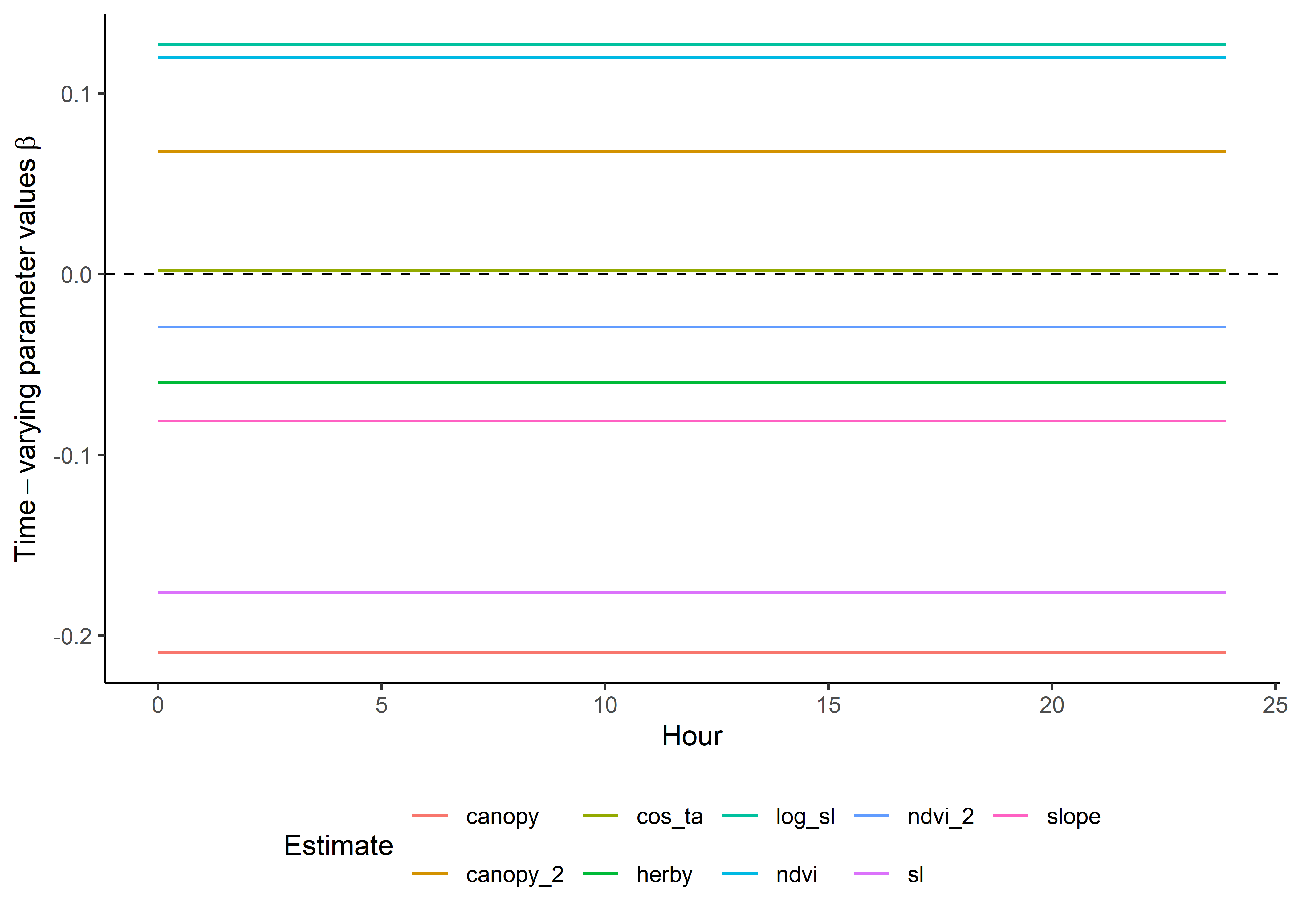
Code
ggplot() +
    geom_path(data = harmonics_scaled_long_1p,
              aes(x = hour, y = value, colour = coef)) +
    geom_hline(yintercept = 0, linetype = "dashed") +
    scale_y_continuous(expression(Time-varying~parameter~values~beta)) +
    scale_x_continuous("Hour") +
    scale_color_discrete("Estimate") +
    theme_classic() +
    theme(legend.position = "bottom")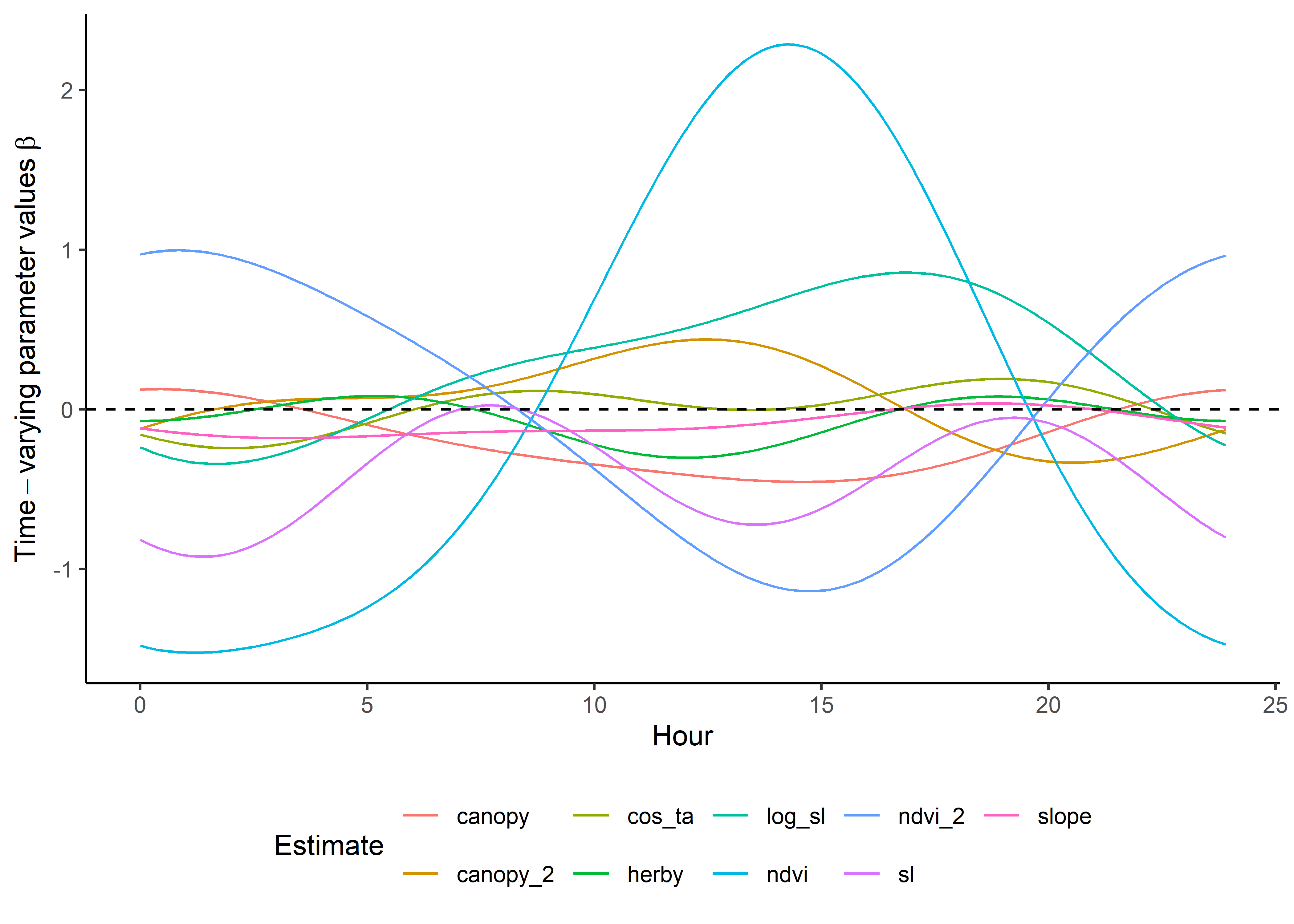
Code
ggplot() +
    geom_path(data = harmonics_scaled_long_2p,
              aes(x = hour, y = value, colour = coef)) +
    geom_hline(yintercept = 0, linetype = "dashed") +
    scale_y_continuous(expression(Time-varying~parameter~values~beta)) +
    scale_x_continuous("Hour") +
    scale_color_discrete("Estimate") +
    theme_classic() +
    theme(legend.position = "bottom")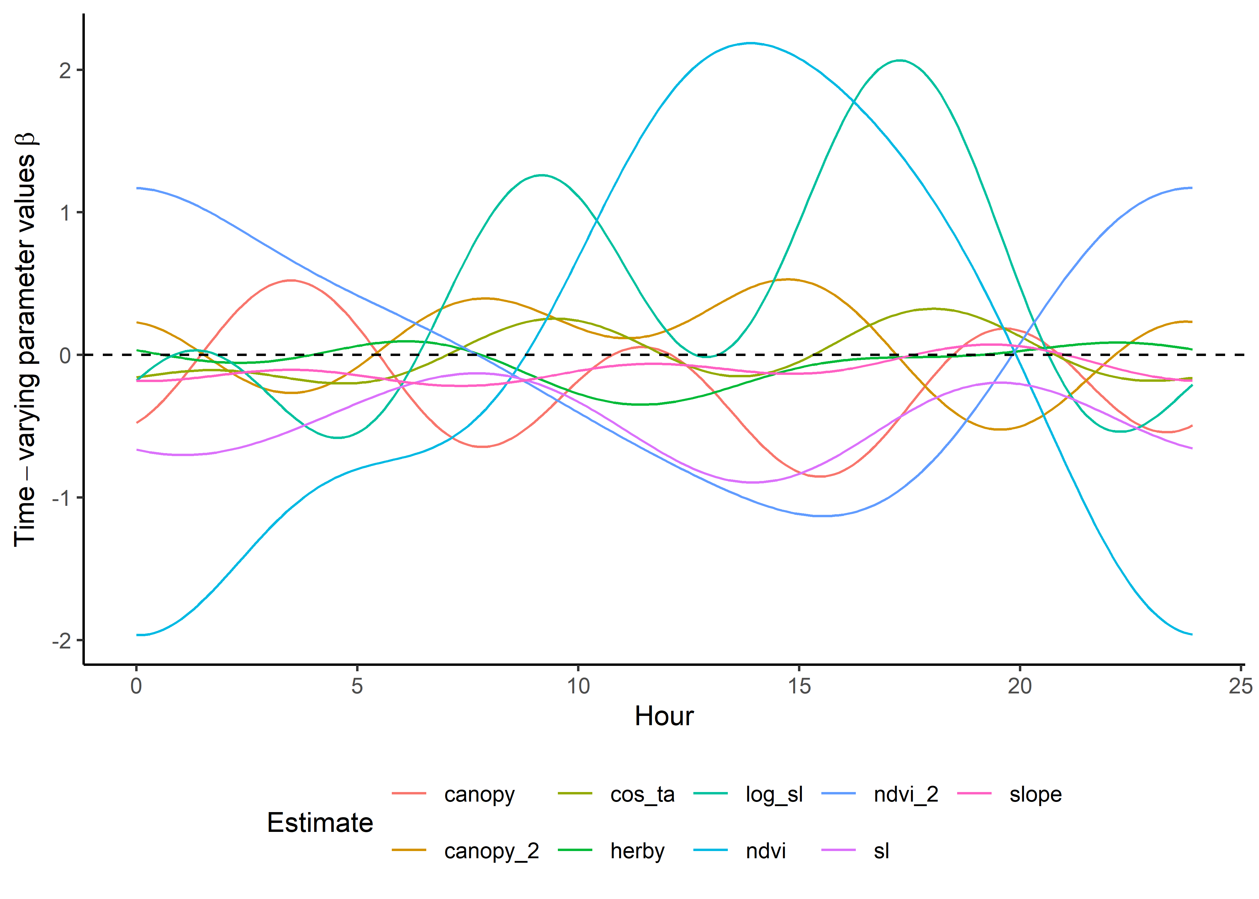
Code
ggplot() +
    geom_path(data = harmonics_scaled_long_3p,
              aes(x = hour, y = value, colour = coef)) +
    geom_hline(yintercept = 0, linetype = "dashed") +
    scale_y_continuous(expression(Time-varying~parameter~values~beta)) +
    scale_x_continuous("Hour") +
    scale_color_discrete("Estimate") +
    theme_classic() +
    theme(legend.position = "bottom")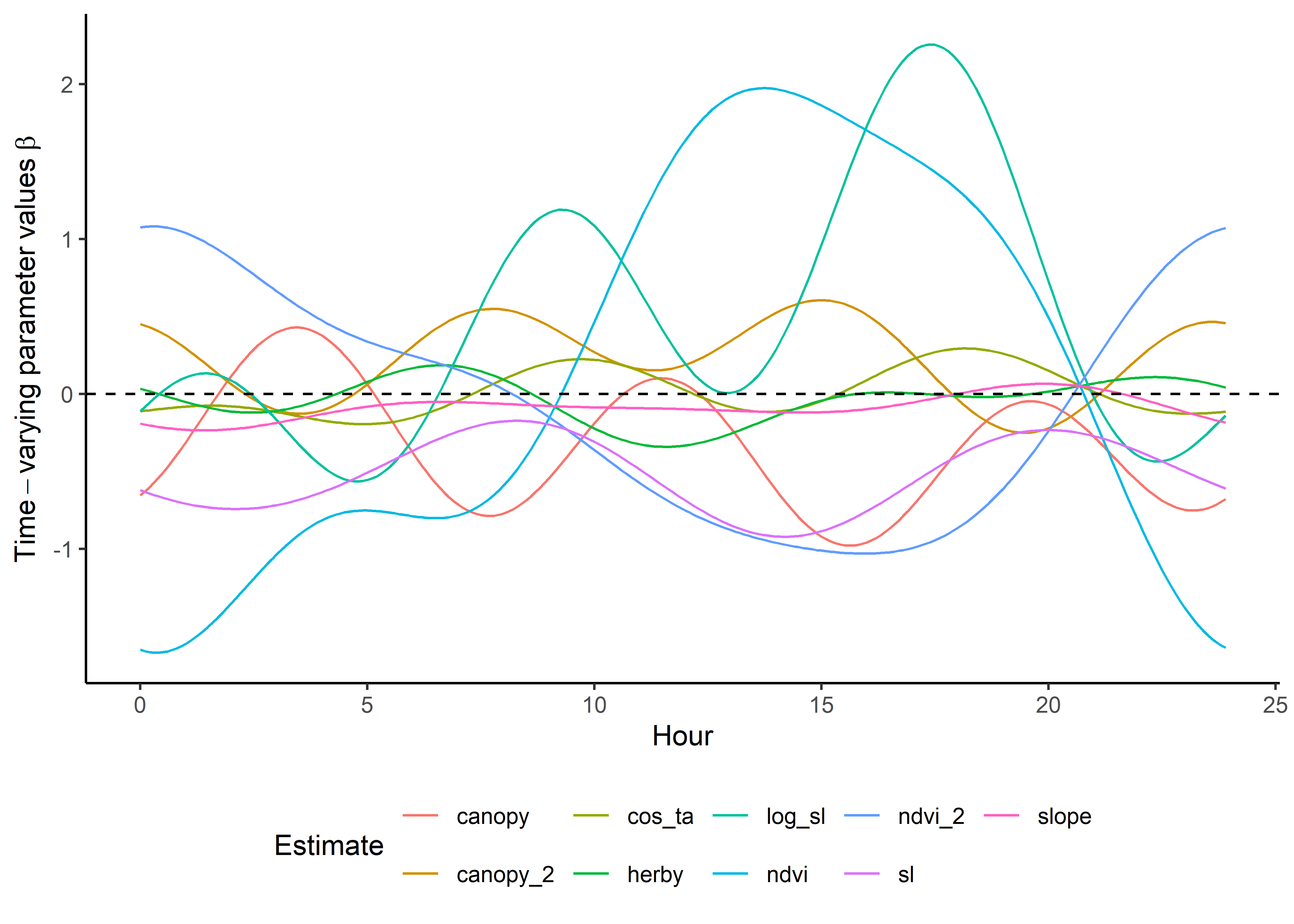
Reconstructing the natural-scale temporally dynamic coefficients
As we scaled the covariate values prior to fitting the models, we want to rescale the coefficients to their natural scale. This is important for the simulations, as the environmental variables will not be scaled when we simulate steps.
Code
harmonics_nat_df_0p <- data.frame(
  "hour" = hour,
  "ndvi" = as.numeric(
    coefs_clr_0p %>% dplyr::filter(grepl("ndvi", coefs) & !grepl("sq", coefs)) %>%
      pull(value_nat) %>% t() %*% t(as.matrix(hour_harmonics_df_0p))),
  "ndvi_2" = as.numeric(
    coefs_clr_0p %>% dplyr::filter(grepl("ndvi_sq", coefs)) %>%
      pull(value_nat) %>% t() %*% t(as.matrix(hour_harmonics_df_0p))),
  "canopy" = as.numeric(
    coefs_clr_0p %>% dplyr::filter(grepl("canopy", coefs) & !grepl("sq", coefs)) %>%
      pull(value_nat) %>% t() %*% t(as.matrix(hour_harmonics_df_0p))),
  "canopy_2" = as.numeric(
    coefs_clr_0p %>% dplyr::filter(grepl("canopy_sq", coefs)) %>%
      pull(value_nat) %>% t() %*% t(as.matrix(hour_harmonics_df_0p))),
  "slope" = as.numeric(
    coefs_clr_0p %>% dplyr::filter(grepl("slope", coefs) & !grepl("sq", coefs)) %>%
      pull(value_nat) %>% t() %*% t(as.matrix(hour_harmonics_df_0p))),
  "herby" = as.numeric(
    coefs_clr_0p %>% dplyr::filter(grepl("herby", coefs)) %>%
      pull(value_nat) %>% t() %*% t(as.matrix(hour_harmonics_df_0p))),
  "sl" = as.numeric(
    coefs_clr_0p %>% dplyr::filter(grepl("step_l", coefs) & !grepl("log", coefs)) %>%
      pull(value_nat) %>% t() %*% t(as.matrix(hour_harmonics_df_0p))),
  "log_sl" = as.numeric(
    coefs_clr_0p %>% dplyr::filter(grepl("log_step_l", coefs)) %>%
      pull(value_nat) %>% t() %*% t(as.matrix(hour_harmonics_df_0p))),
  "cos_ta" = as.numeric(
    coefs_clr_0p %>% dplyr::filter(grepl("cos", coefs)) %>%
      pull(value_nat) %>% t() %*% t(as.matrix(hour_harmonics_df_0p))))
Code
harmonics_nat_df_1p <- data.frame(
  "hour" = hour,
  "ndvi" = as.numeric(
    coefs_clr_1p %>% dplyr::filter(grepl("ndvi", coefs) & !grepl("sq", coefs)) %>%
      pull(value_nat) %>% t() %*% t(as.matrix(hour_harmonics_df_1p))),
  "ndvi_2" = as.numeric(
    coefs_clr_1p %>% dplyr::filter(grepl("ndvi_sq", coefs)) %>%
      pull(value_nat) %>% t() %*% t(as.matrix(hour_harmonics_df_1p))),
  "canopy" = as.numeric(
    coefs_clr_1p %>% dplyr::filter(grepl("canopy", coefs) & !grepl("sq", coefs)) %>%
      pull(value_nat) %>% t() %*% t(as.matrix(hour_harmonics_df_1p))),
  "canopy_2" = as.numeric(
    coefs_clr_1p %>% dplyr::filter(grepl("canopy_sq", coefs)) %>%
      pull(value_nat) %>% t() %*% t(as.matrix(hour_harmonics_df_1p))),
  "slope" = as.numeric(
    coefs_clr_1p %>% dplyr::filter(grepl("slope", coefs) & !grepl("sq", coefs)) %>%
      pull(value_nat) %>% t() %*% t(as.matrix(hour_harmonics_df_1p))),
  "herby" = as.numeric(
    coefs_clr_1p %>% dplyr::filter(grepl("herby", coefs)) %>%
      pull(value_nat) %>% t() %*% t(as.matrix(hour_harmonics_df_1p))),
  "sl" = as.numeric(
    coefs_clr_1p %>% dplyr::filter(grepl("step_l", coefs) & !grepl("log", coefs)) %>%
      pull(value_nat) %>% t() %*% t(as.matrix(hour_harmonics_df_1p))),
  "log_sl" = as.numeric(
    coefs_clr_1p %>% dplyr::filter(grepl("log_step_l", coefs)) %>%
      pull(value_nat) %>% t() %*% t(as.matrix(hour_harmonics_df_1p))),
  "cos_ta" = as.numeric(
    coefs_clr_1p %>% dplyr::filter(grepl("cos", coefs)) %>%
      pull(value_nat) %>% t() %*% t(as.matrix(hour_harmonics_df_1p))))
Code
harmonics_nat_df_2p <- data.frame(
  "hour" = hour,
  "ndvi" = as.numeric(
    coefs_clr_2p %>% dplyr::filter(grepl("ndvi", coefs) & !grepl("sq", coefs)) %>%
      pull(value_nat) %>% t() %*% t(as.matrix(hour_harmonics_df_2p))),
  "ndvi_2" = as.numeric(
    coefs_clr_2p %>% dplyr::filter(grepl("ndvi_sq", coefs)) %>%
      pull(value_nat) %>% t() %*% t(as.matrix(hour_harmonics_df_2p))),
  "canopy" = as.numeric(
    coefs_clr_2p %>% dplyr::filter(grepl("canopy", coefs) & !grepl("sq", coefs)) %>%
      pull(value_nat) %>% t() %*% t(as.matrix(hour_harmonics_df_2p))),
  "canopy_2" = as.numeric(
    coefs_clr_2p %>% dplyr::filter(grepl("canopy_sq", coefs)) %>%
      pull(value_nat) %>% t() %*% t(as.matrix(hour_harmonics_df_2p))),
  "slope" = as.numeric(
    coefs_clr_2p %>% dplyr::filter(grepl("slope", coefs) & !grepl("sq", coefs)) %>%
      pull(value_nat) %>% t() %*% t(as.matrix(hour_harmonics_df_2p))),
  "herby" = as.numeric(
    coefs_clr_2p %>% dplyr::filter(grepl("herby", coefs)) %>%
      pull(value_nat) %>% t() %*% t(as.matrix(hour_harmonics_df_2p))),
  "sl" = as.numeric(
    coefs_clr_2p %>% dplyr::filter(grepl("step_l", coefs) & !grepl("log", coefs)) %>%
      pull(value_nat) %>% t() %*% t(as.matrix(hour_harmonics_df_2p))),
  "log_sl" = as.numeric(
    coefs_clr_2p %>% dplyr::filter(grepl("log_step_l", coefs)) %>%
      pull(value_nat) %>% t() %*% t(as.matrix(hour_harmonics_df_2p))),
  "cos_ta" = as.numeric(
    coefs_clr_2p %>% dplyr::filter(grepl("cos", coefs)) %>%
      pull(value_nat) %>% t() %*% t(as.matrix(hour_harmonics_df_2p))))
Code
harmonics_nat_df_3p <- data.frame(
  "hour" = hour,
  "ndvi" = as.numeric(
    coefs_clr_3p %>% dplyr::filter(grepl("ndvi", coefs) & !grepl("sq", coefs)) %>%
      pull(value_nat) %>% t() %*% t(as.matrix(hour_harmonics_df_3p))),
  "ndvi_2" = as.numeric(
    coefs_clr_3p %>% dplyr::filter(grepl("ndvi_sq", coefs)) %>%
      pull(value_nat) %>% t() %*% t(as.matrix(hour_harmonics_df_3p))),
  "canopy" = as.numeric(
    coefs_clr_3p %>% dplyr::filter(grepl("canopy", coefs) & !grepl("sq", coefs)) %>%
      pull(value_nat) %>% t() %*% t(as.matrix(hour_harmonics_df_3p))),
  "canopy_2" = as.numeric(
    coefs_clr_3p %>% dplyr::filter(grepl("canopy_sq", coefs)) %>%
      pull(value_nat) %>% t() %*% t(as.matrix(hour_harmonics_df_3p))),
  "slope" = as.numeric(
    coefs_clr_3p %>% dplyr::filter(grepl("slope", coefs) & !grepl("sq", coefs)) %>%
      pull(value_nat) %>% t() %*% t(as.matrix(hour_harmonics_df_3p))),
  "herby" = as.numeric(
    coefs_clr_3p %>% dplyr::filter(grepl("herby", coefs)) %>%
      pull(value_nat) %>% t() %*% t(as.matrix(hour_harmonics_df_3p))),
  "sl" = as.numeric(
    coefs_clr_3p %>% dplyr::filter(grepl("step_l", coefs) & !grepl("log", coefs)) %>%
      pull(value_nat) %>% t() %*% t(as.matrix(hour_harmonics_df_3p))),
  "log_sl" = as.numeric(
    coefs_clr_3p %>% dplyr::filter(grepl("log_step_l", coefs)) %>%
      pull(value_nat) %>% t() %*% t(as.matrix(hour_harmonics_df_3p))),
  "cos_ta" = as.numeric(
    coefs_clr_3p %>% dplyr::filter(grepl("cos", coefs)) %>%
      pull(value_nat) %>% t() %*% t(as.matrix(hour_harmonics_df_3p))))
Update the Gamma and von Mises distributions
To update the Gamma and von Mises distribution from the tentative distributions (e.g. Fieberg et al. 2021, Appendix C), we just do the calculation at each time point (for the natural-scale coefficients).
Code
# from the step generation script
tentative_shape <- 0.438167
tentative_scale <- 534.3507
tentative_kappa <- 0.1848126

hour_coefs_nat_df_0p <- harmonics_nat_df_0p %>%
  mutate(shape = tentative_shape + log_sl,
         scale = 1/((1/tentative_scale) - sl),
         kappa = tentative_kappa + cos_ta)

# save the coefficients to use in the simulations
write_csv(hour_coefs_nat_df_0p,
          paste0("ssf_coefficients/id", focal_id, "_0pDaily_coefs_80-10-10_", Sys.Date(), ".csv"))

# turning into a long data frame
hour_coefs_nat_long_0p <- pivot_longer(hour_coefs_nat_df_0p,
                                       cols = !1,
                                       names_to = "coef")
Code
hour_coefs_nat_df_1p <- harmonics_nat_df_1p %>%
  mutate(shape = tentative_shape + log_sl,
         scale = 1/((1/tentative_scale) - sl),
         kappa = tentative_kappa + cos_ta)

# save the coefficients to use in the simulations
write_csv(hour_coefs_nat_df_1p,
          paste0("ssf_coefficients/id", focal_id, "_1pDaily_coefs_80-10-10_",Sys.Date(), ".csv"))

# turning into a long data frame
hour_coefs_nat_long_1p <- pivot_longer(hour_coefs_nat_df_1p,
                                       cols = !1, names_to = "coef")
Code
hour_coefs_nat_df_2p <- harmonics_nat_df_2p %>%
  mutate(shape = tentative_shape + log_sl,
         scale = 1/((1/tentative_scale) - sl),
         kappa = tentative_kappa + cos_ta)

# save the coefficients to use in the simulations
write_csv(hour_coefs_nat_df_2p,
          paste0("ssf_coefficients/id", focal_id, "_2pDaily_coefs_80-10-10_",Sys.Date(), ".csv"))

# turning into a long data frame
hour_coefs_nat_long_2p <- pivot_longer(hour_coefs_nat_df_2p, cols = !1,
                                       names_to = "coef")
Code
hour_coefs_nat_df_3p <- harmonics_nat_df_3p %>%
  mutate(shape = tentative_shape + log_sl,
         scale = 1/((1/tentative_scale) - sl),
         kappa = tentative_kappa + cos_ta)

# save the coefficients to use in the simulations
write_csv(hour_coefs_nat_df_3p,
          paste0("ssf_coefficients/id", focal_id, "_3pDaily_coefs_80-10-10_", Sys.Date(), ".csv"))

# turning into a long data frame
hour_coefs_nat_long_3p <- pivot_longer(hour_coefs_nat_df_3p, cols = !1,
                                       names_to = "coef")
Plot the natural-scale temporally dynamic coefficients
Now that the coefficients are in their natural scales, they will be larger or smaller depending on the scale of the covariate.
Plot just the habitat selection coefficients.
Code
ggplot() +
  geom_path(data = hour_coefs_nat_long_0p %>%
              filter(!coef %in% c("shape", "scale", "kappa")),
            aes(x = hour, y = value, colour = coef)) +
  geom_hline(yintercept = 0, linetype = "dashed") +
  scale_y_continuous(expression(Time-varying~parameter~values~beta)) +
  scale_x_continuous("Hour", breaks = seq(0,24,2)) +
  scale_color_discrete("Estimate") +
  theme_classic() +
  theme(legend.position = "bottom")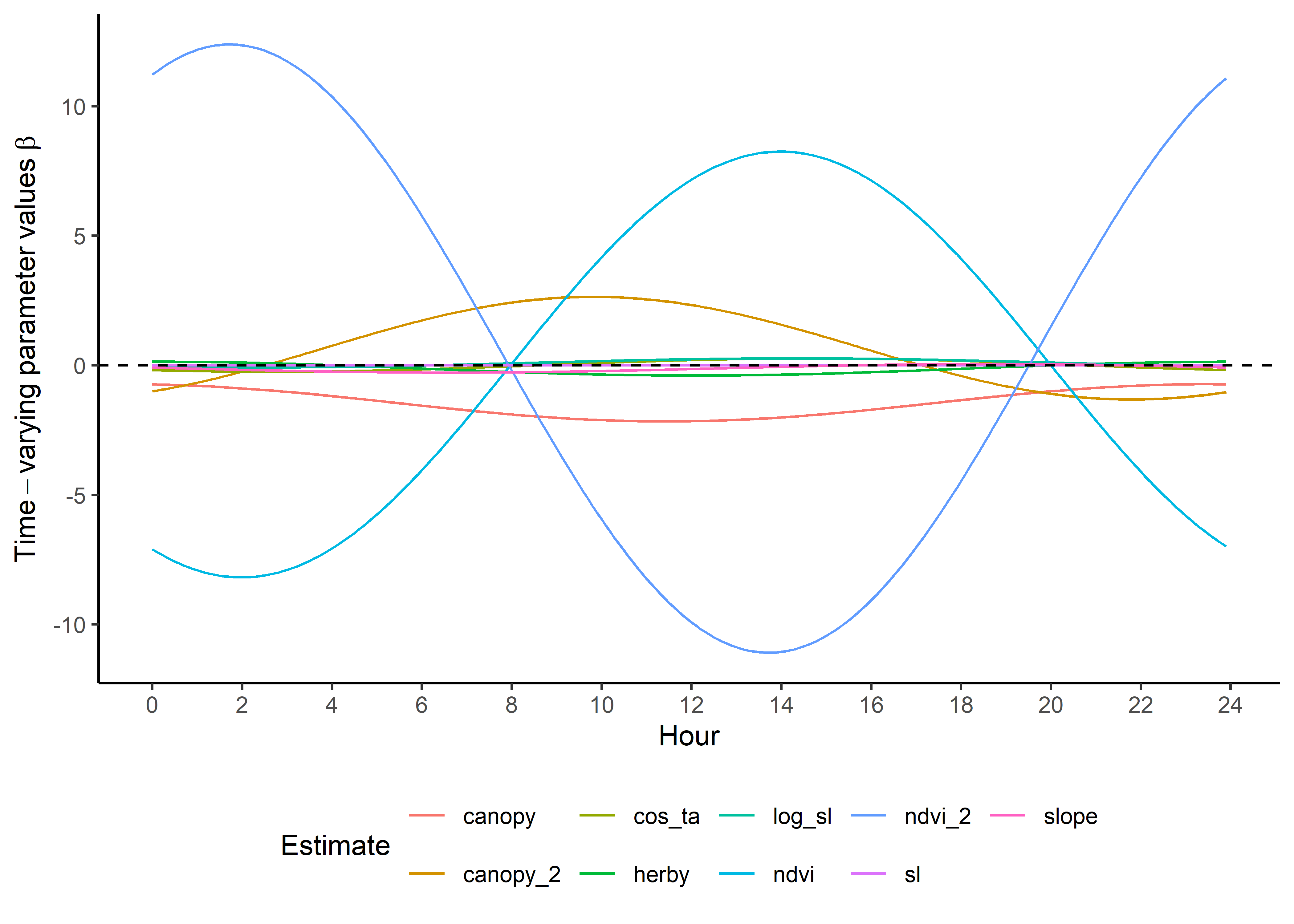
Code
ggplot() +
  geom_path(data = hour_coefs_nat_long_1p %>%
              filter(!coef %in% c("shape", "scale", "kappa")),
            aes(x = hour, y = value, colour = coef)) +
  geom_hline(yintercept = 0, linetype = "dashed") +
  scale_y_continuous(expression(Time-varying~parameter~values~beta)) +
  scale_x_continuous("Hour", breaks = seq(0,24,2)) +
  scale_color_discrete("Estimate") +
  theme_classic() +
  theme(legend.position = "bottom")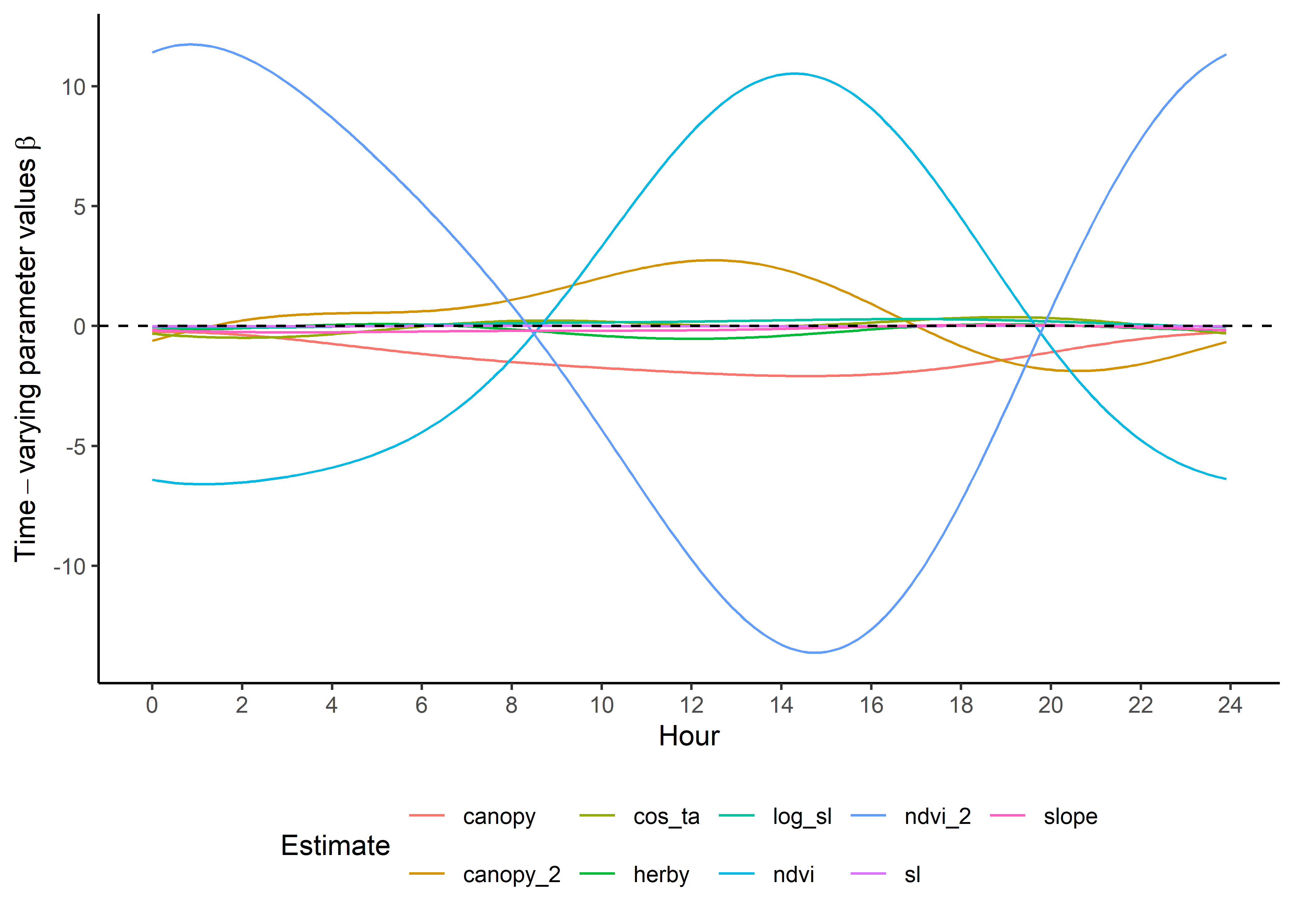
Code
ggplot() +
  geom_path(data = hour_coefs_nat_long_2p %>%
              filter(!coef %in% c("shape", "scale", "kappa")),
            aes(x = hour, y = value, colour = coef)) +
  geom_hline(yintercept = 0, linetype = "dashed") +
  scale_y_continuous(expression(Time-varying~parameter~values~beta)) +
  scale_x_continuous("Hour", breaks = seq(0,24,2)) +
  scale_color_discrete("Estimate") +
  theme_classic() +
  theme(legend.position = "bottom")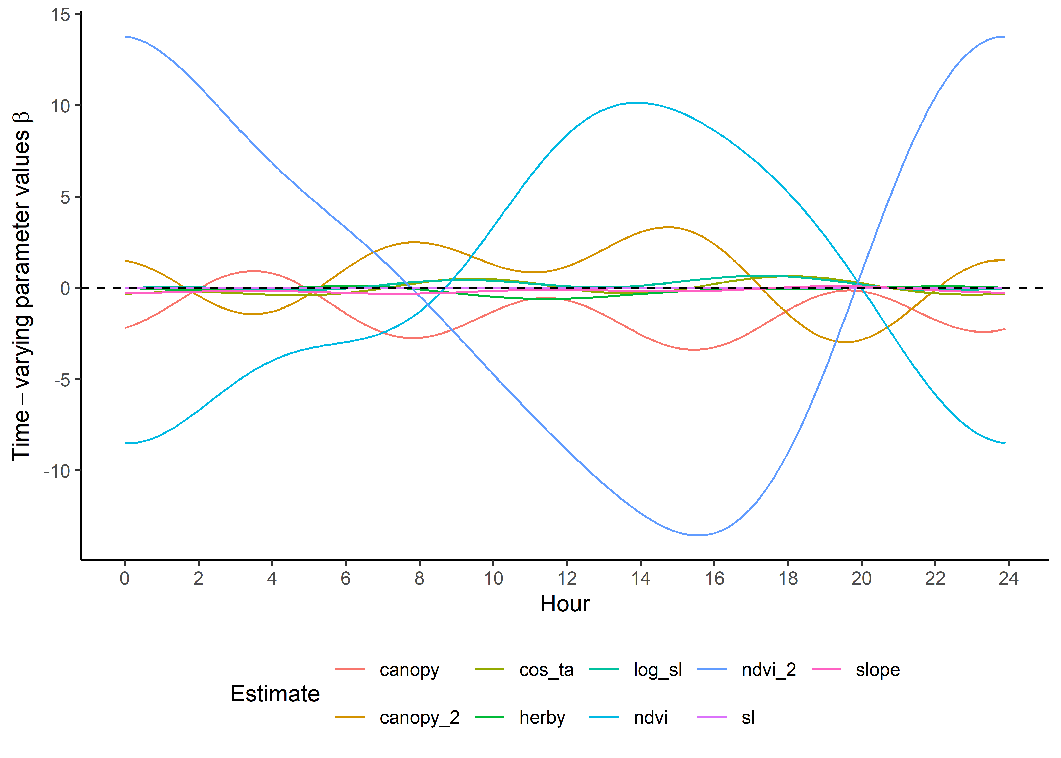
Code
ggplot() +
  geom_path(data = hour_coefs_nat_long_3p %>%
              filter(!coef %in% c("shape", "scale", "kappa")),
            aes(x = hour, y = value, colour = coef)) +
  geom_hline(yintercept = 0, linetype = "dashed") +
  scale_y_continuous(expression(Time-varying~parameter~values~beta)) +
  scale_x_continuous("Hour", breaks = seq(0,24,2)) +
  scale_color_discrete("Estimate") +
  theme_classic() +
  theme(legend.position = "bottom")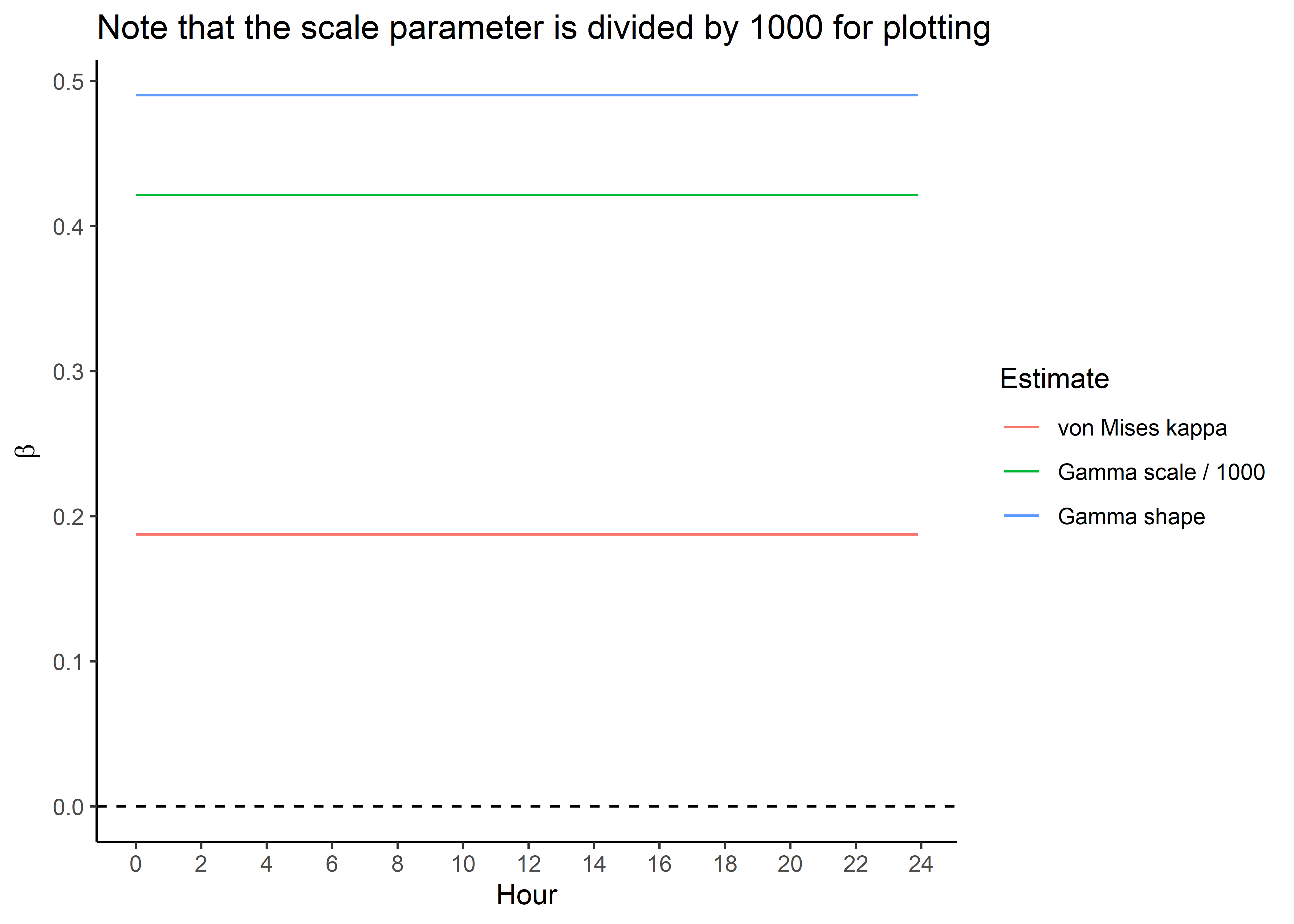
Plot only the temporally dynamic movement parameters
Code
ggplot() +
    geom_path(data = hour_coefs_nat_long_0p %>%
              filter(coef %in% c("shape", "kappa")),
              aes(x = hour, y = value, colour = coef)) +
  geom_path(data = hour_coefs_nat_long_0p %>%
              filter(coef == "scale"),
              aes(x = hour, y = value/1000, colour = coef)) +
    geom_hline(yintercept = 0, linetype = "dashed") +
    scale_y_continuous(expression(beta)) +
  scale_x_continuous("Hour", breaks = seq(0,24,2)) +
  ggtitle("Note that the scale parameter is divided by 1000 for plotting") +
  scale_color_discrete("Estimate",
      labels = c("kappa" = "von Mises kappa",
                 "scale" = "Gamma scale / 1000",
                 "shape" = "Gamma shape")) +
    theme_classic() +
    theme(legend.position = "right")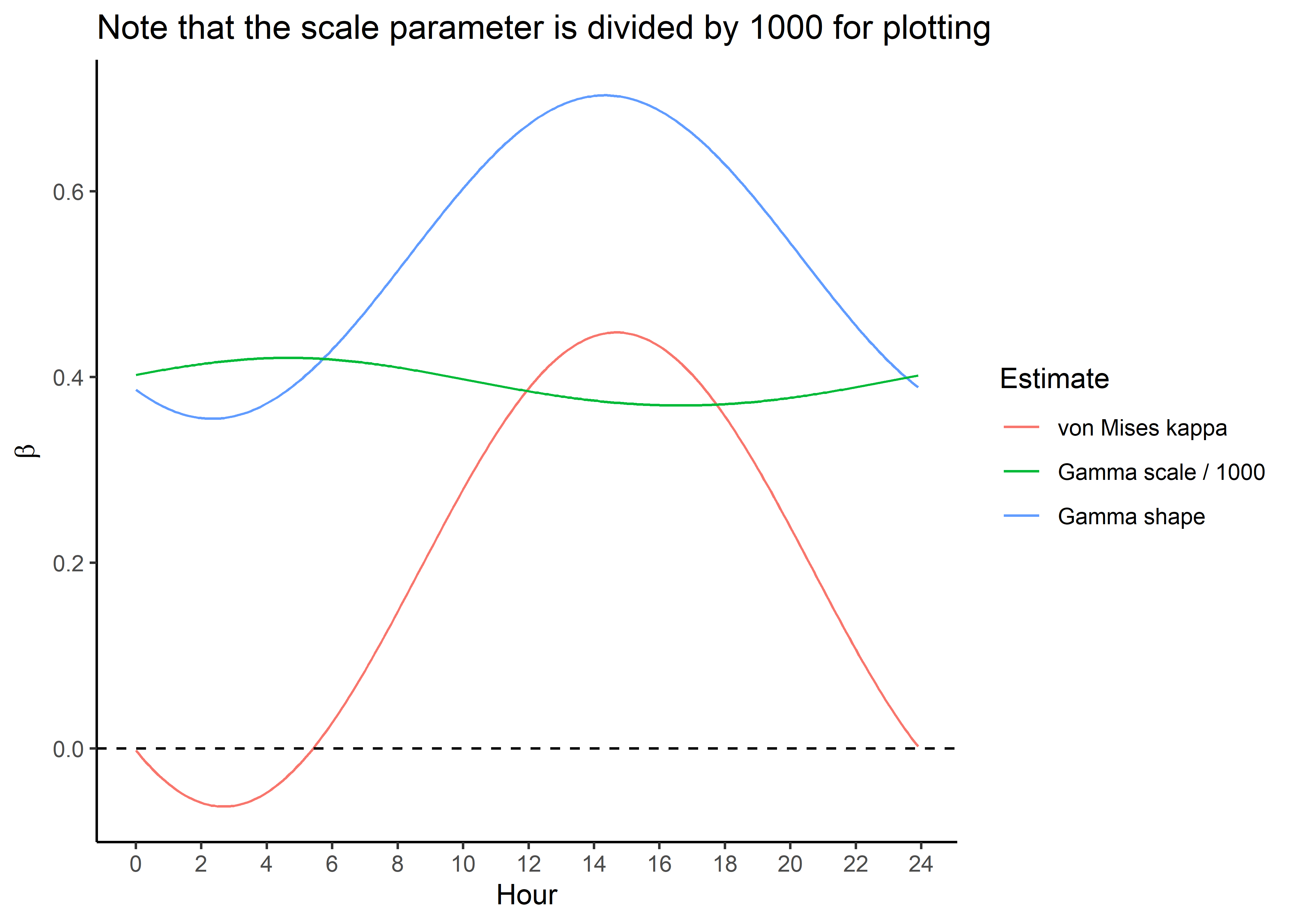
Code
ggplot() +
    geom_path(data = hour_coefs_nat_long_1p %>%
              filter(coef %in% c("shape", "kappa")),
              aes(x = hour, y = value, colour = coef)) +
  geom_path(data = hour_coefs_nat_long_1p %>%
              filter(coef == "scale"),
              aes(x = hour, y = value/1000, colour = coef)) +
    geom_hline(yintercept = 0, linetype = "dashed") +
    scale_y_continuous(expression(beta)) +
  scale_x_continuous("Hour", breaks = seq(0,24,2)) +
  ggtitle("Note that the scale parameter is divided by 1000 for plotting") +
  scale_color_discrete("Estimate",
      labels = c("kappa" = "von Mises kappa",
                 "scale" = "Gamma scale / 1000",
                 "shape" = "Gamma shape")) +
    theme_classic() +
    theme(legend.position = "right")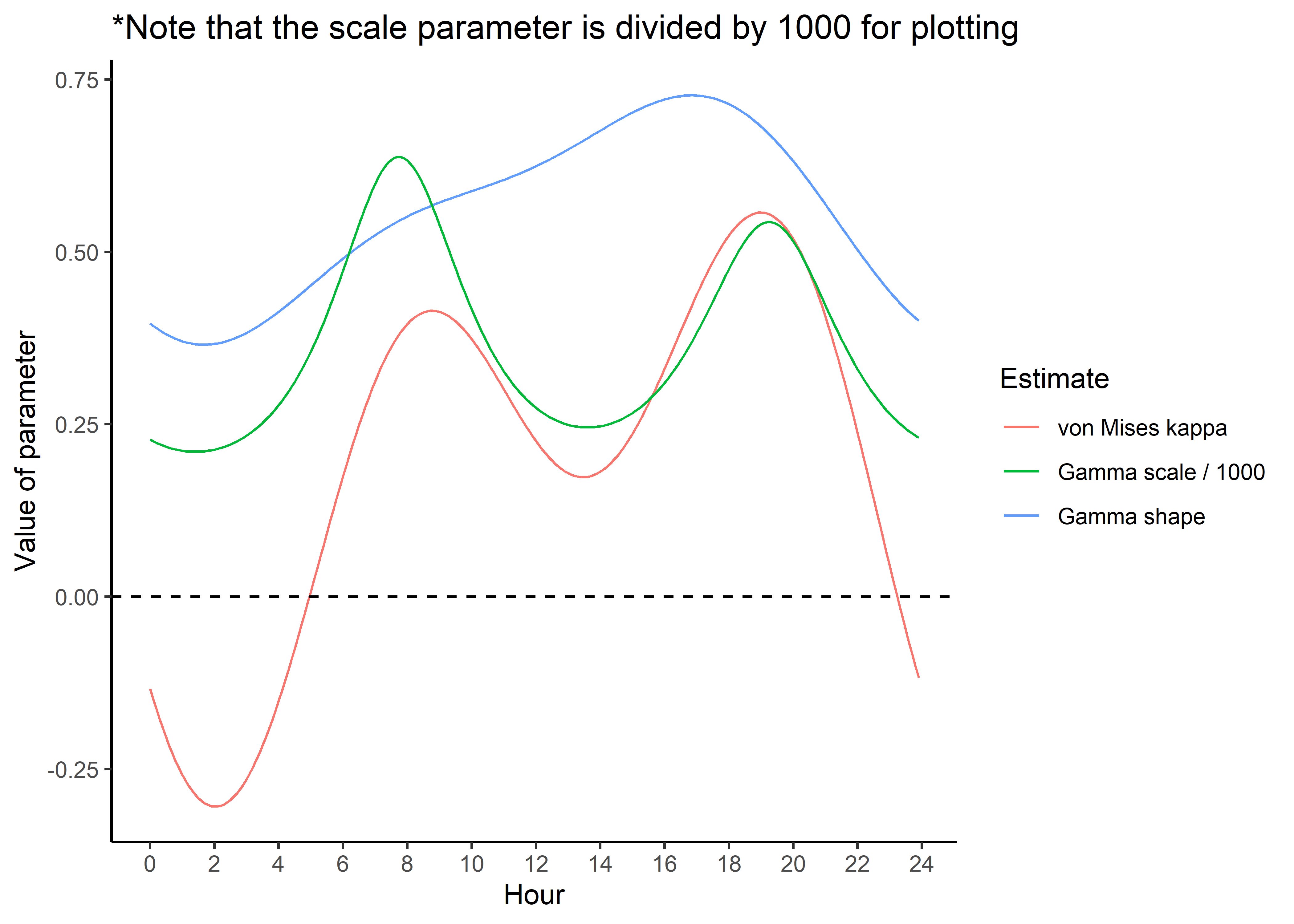
Code
ggplot() +
    geom_path(data = hour_coefs_nat_long_2p %>%
              filter(coef %in% c("shape", "kappa")),
              aes(x = hour, y = value, colour = coef)) +
  geom_path(data = hour_coefs_nat_long_2p %>%
              filter(coef == "scale"),
              aes(x = hour, y = value/1000, colour = coef)) +
    geom_hline(yintercept = 0, linetype = "dashed") +
    scale_y_continuous("Value of parameter") +
  scale_x_continuous("Hour", breaks = seq(0,24,2)) +
  ggtitle("*Note that the scale parameter is divided by 1000 for plotting") +
  scale_color_discrete("Estimate",
      labels = c("kappa" = "von Mises kappa",
                 "scale" = "Gamma scale / 1000",
                 "shape" = "Gamma shape")) +
    theme_classic() +
    theme(legend.position = "right")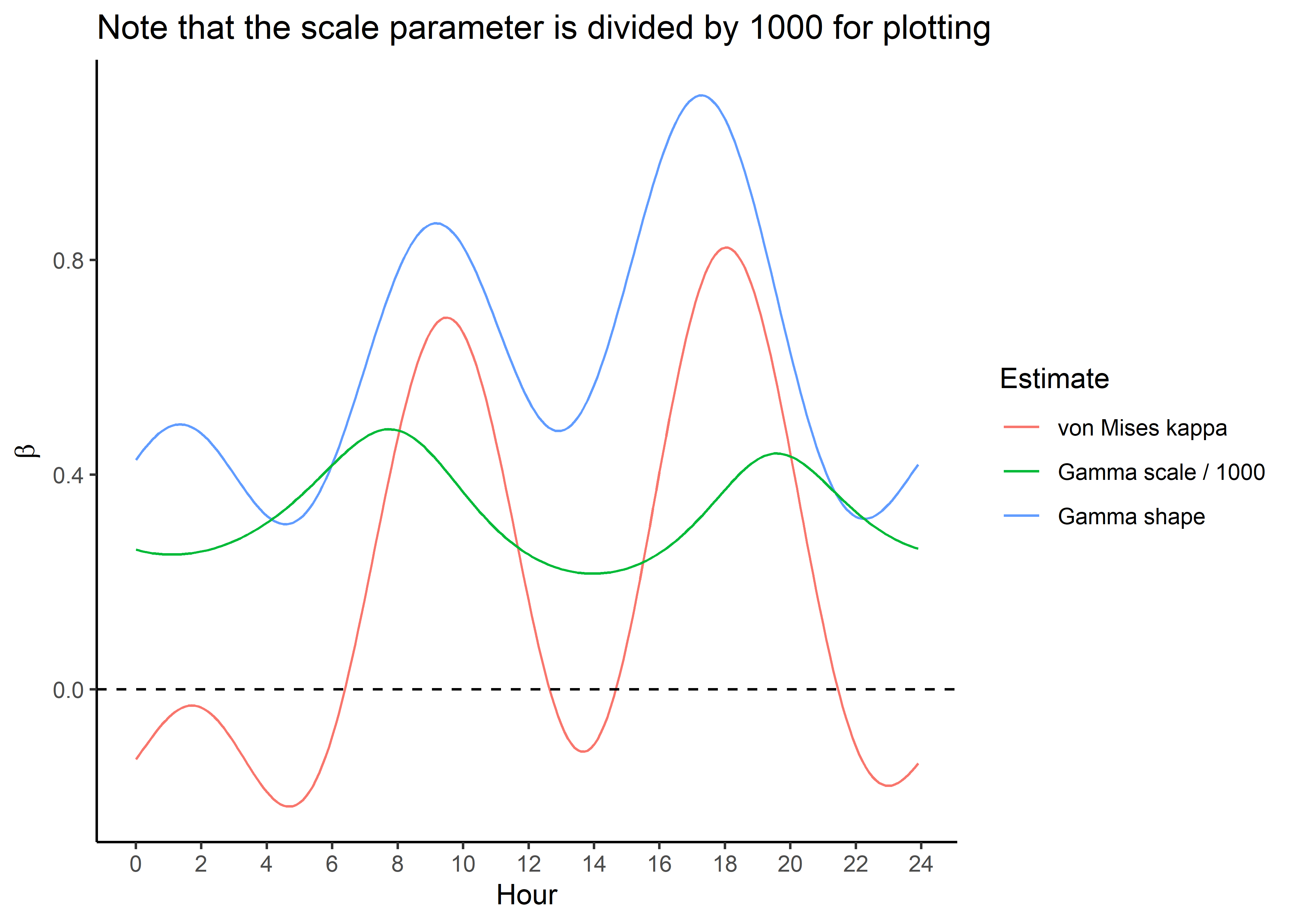
Code
ggplot() +
    geom_path(data = hour_coefs_nat_long_3p %>%
              filter(coef %in% c("shape", "kappa")),
              aes(x = hour, y = value, colour = coef)) +
  geom_path(data = hour_coefs_nat_long_3p %>%
              filter(coef == "scale"),
              aes(x = hour, y = value/1000, colour = coef)) +
    geom_hline(yintercept = 0, linetype = "dashed") +
    scale_y_continuous(expression(beta)) +
  scale_x_continuous("Hour", breaks = seq(0,24,2)) +
  ggtitle("Note that the scale parameter is divided by 1000 for plotting") +
  scale_color_discrete("Estimate",
      labels = c("kappa" = "von Mises kappa",
                 "scale" = "Gamma scale / 1000",
                 "shape" = "Gamma shape")) +
    theme_classic() +
    theme(legend.position = "right")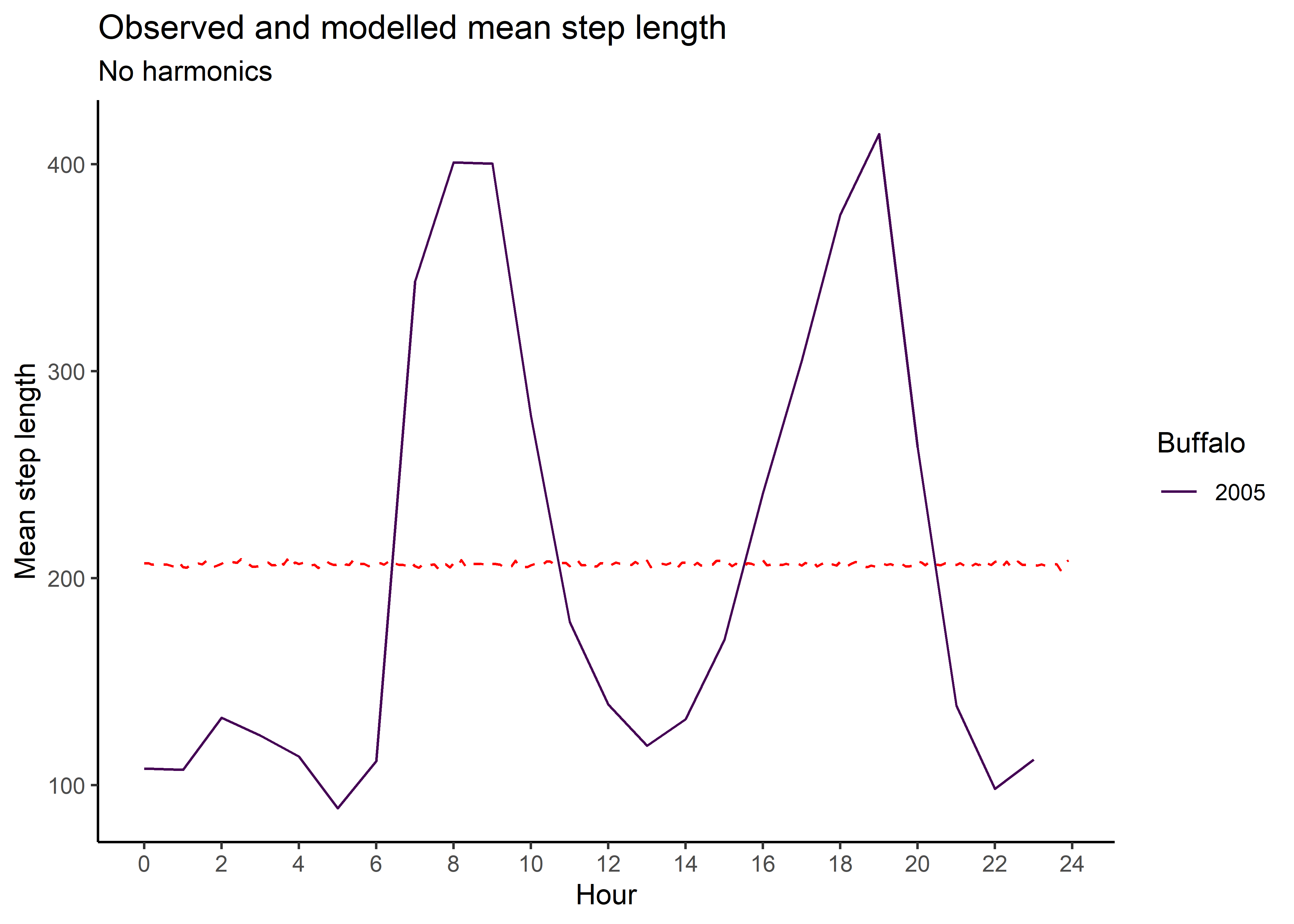
Sample from temporally dynamic movement parameters
Here we sample from the movement kernel to generate a distribution of step lengths for each hour of the day, to assess how well it matches the observed step lengths. This is the ‘selection-free’ movement kernel, so the step lengths and turning angles from the simulations will be different, as the steps will be conditioned on the habitat, but this is a useful diagnostic to assess whether the harmonics are capturing the observed movement dynamics.
Code
`summarise()` has grouped output by 'id'. You can override using the `.groups`
argument.
Code
# number of samples at each hour (more = smoother plotting, but slower)
n <- 1e5

gamma_dist_list <- vector(mode = "list", length = nrow(hour_coefs_nat_df_0p))
gamma_mean <- c()
gamma_median <- c()
gamma_ratio <- c()

for(hour_no in 1:nrow(hour_coefs_nat_df_0p)) {

  gamma_dist_list[[hour_no]] <- rgamma(n, shape = hour_coefs_nat_df_0p$shape[hour_no],
                                       scale = hour_coefs_nat_df_0p$scale[hour_no])

  gamma_mean[hour_no] <- mean(gamma_dist_list[[hour_no]])
  gamma_median[hour_no] <- median(gamma_dist_list[[hour_no]])
  gamma_ratio[hour_no] <- gamma_mean[hour_no] / gamma_median[hour_no]

}

gamma_df_0p <- data.frame(model = "0p",
                          hour = hour_coefs_nat_df_0p$hour,
                          mean = gamma_mean,
                          median = gamma_median,
                          ratio = gamma_ratio)

mean_sl_0p <- ggplot() +
  geom_path(data = movement_summary_buffalo,
            aes(x = hour, y = mean_sl, colour = factor(id))) +
  geom_path(data = gamma_df_0p,
            aes(x = hour, y = mean), colour = "red", linetype = "dashed") +
  scale_x_continuous("Hour", breaks = seq(0,24,2)) +
  scale_y_continuous("Mean step length") +
  scale_colour_viridis_d("Buffalo") +
  ggtitle("Observed and modelled mean step length",
          subtitle = "No harmonics") +
  theme_classic() +
  theme(legend.position = "right")

mean_sl_0p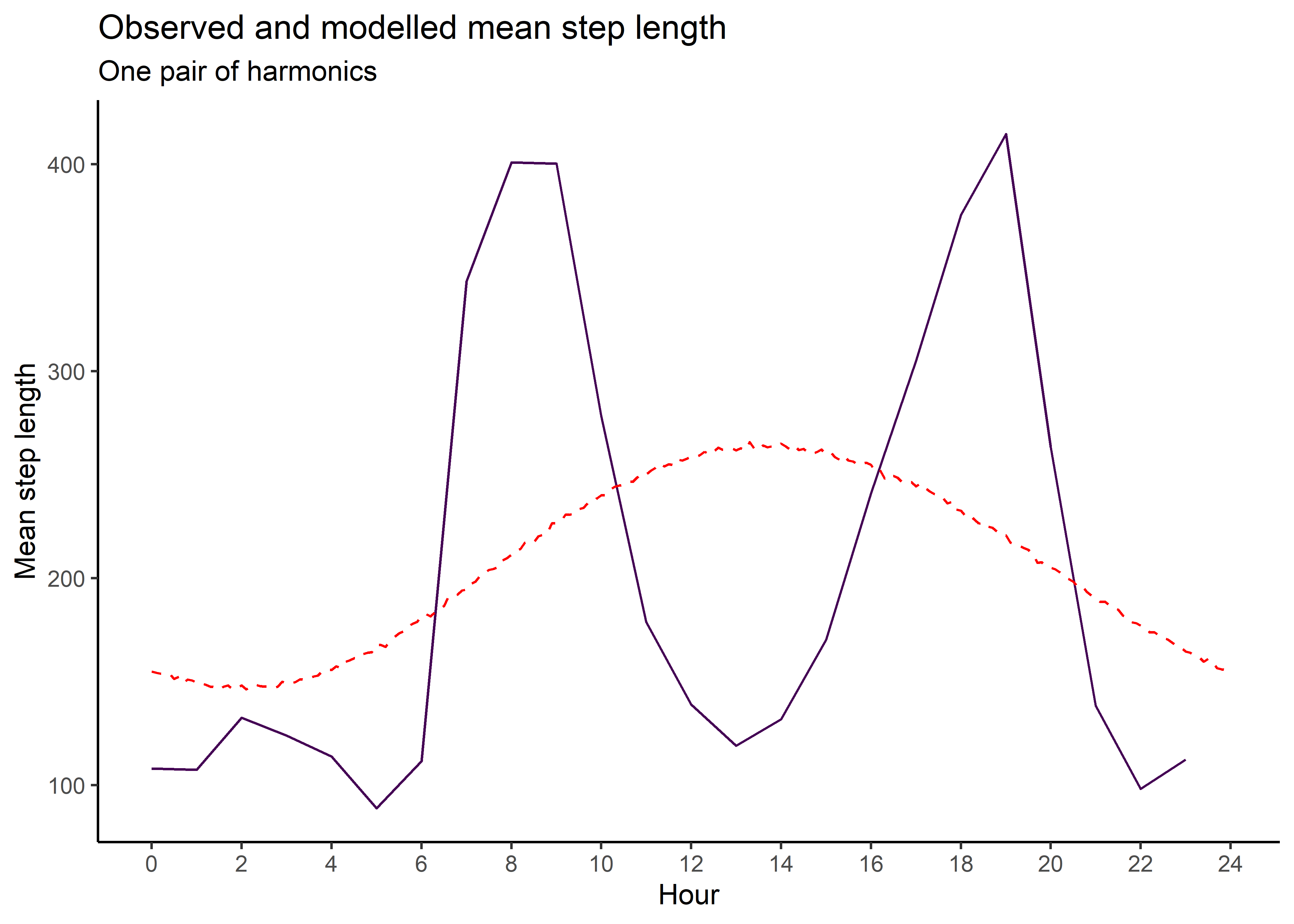
Code
median_sl_0p <- ggplot() +
  geom_path(data = movement_summary_buffalo,
            aes(x = hour, y = median_sl, colour = factor(id))) +
  geom_path(data = gamma_df_0p, aes(x = hour, y = median),
            colour = "red", linetype = "dashed") +
  scale_x_continuous("Hour", breaks = seq(0,24,2)) +
  scale_y_continuous("Median step length") +
  scale_colour_viridis_d("Buffalo") +
  ggtitle("Observed and modelled median step length",
          subtitle = "No harmonics") +
  theme_classic() +
  theme(legend.position = "right")

median_sl_0p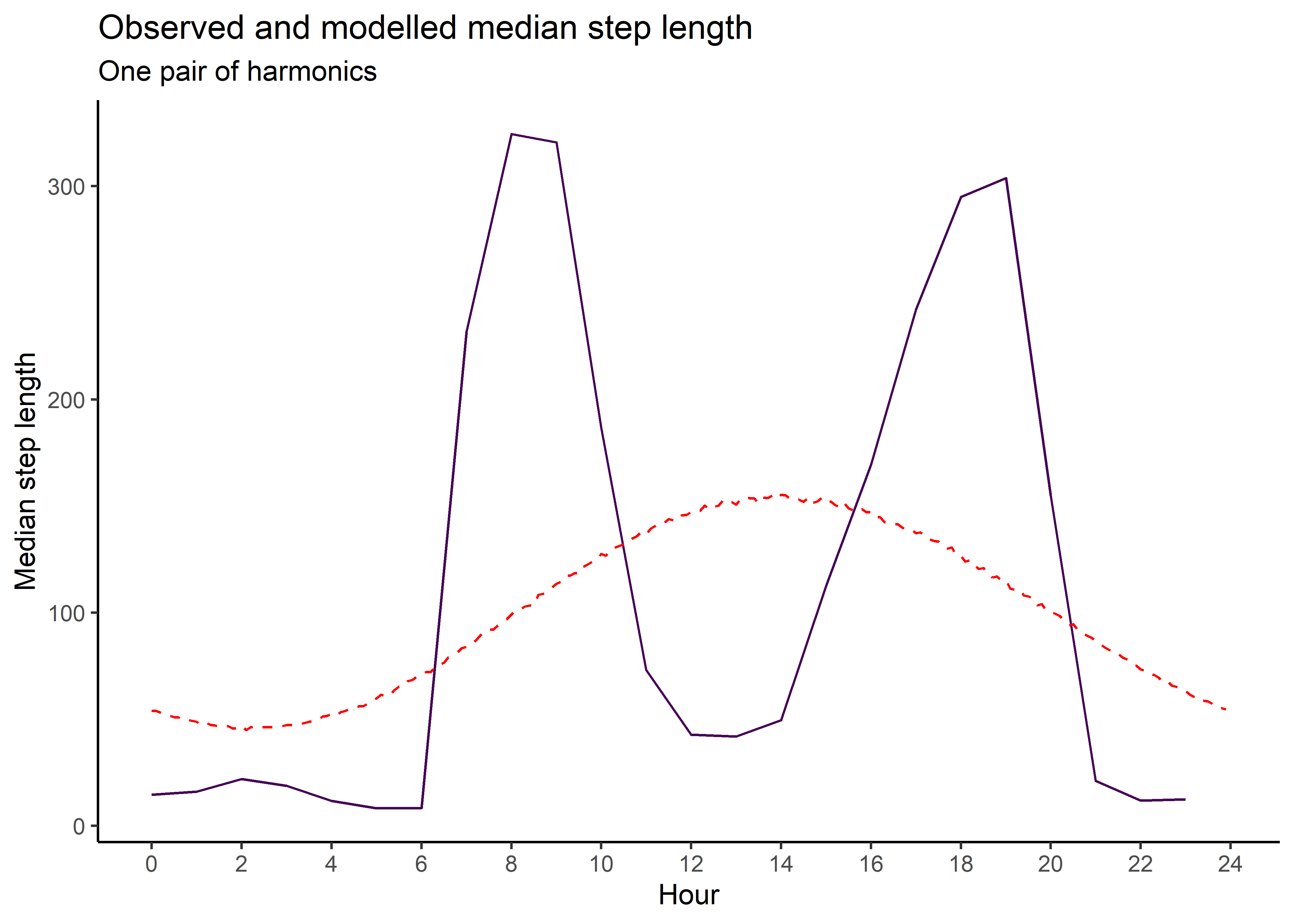
Code
Code
Code
Code
gamma_dist_list <- vector(mode = "list", length = nrow(hour_coefs_nat_df_1p))
gamma_mean <- c()
gamma_median <- c()
gamma_ratio <- c()

for(hour_no in 1:nrow(hour_coefs_nat_df_1p)) {

  gamma_dist_list[[hour_no]] <- rgamma(n,
                                       shape = hour_coefs_nat_df_1p$shape[hour_no],
                                       scale = hour_coefs_nat_df_1p$scale[hour_no])

  gamma_mean[hour_no] <- mean(gamma_dist_list[[hour_no]])
  gamma_median[hour_no] <- median(gamma_dist_list[[hour_no]])
  gamma_ratio[hour_no] <- gamma_mean[hour_no] / gamma_median[hour_no]

}

gamma_df_1p <- data.frame(model = "1p",
                          hour = hour_coefs_nat_df_1p$hour,
                          mean = gamma_mean,
                          median = gamma_median,
                          ratio = gamma_ratio)

mean_sl_1p <- ggplot() +
  geom_path(data = movement_summary_buffalo,
            aes(x = hour, y = mean_sl, colour = factor(id))) +
  geom_path(data = gamma_df_1p,
            aes(x = hour, y = mean),
            colour = "red", linetype = "dashed") +
  scale_x_continuous("Hour", breaks = seq(0,24,2)) +
  scale_y_continuous("Mean step length") +
  scale_colour_viridis_d("Buffalo") +
  ggtitle("Observed and modelled mean step length",
          subtitle = "One pair of harmonics") +
  theme_classic() +
  theme(legend.position = "none")

mean_sl_1p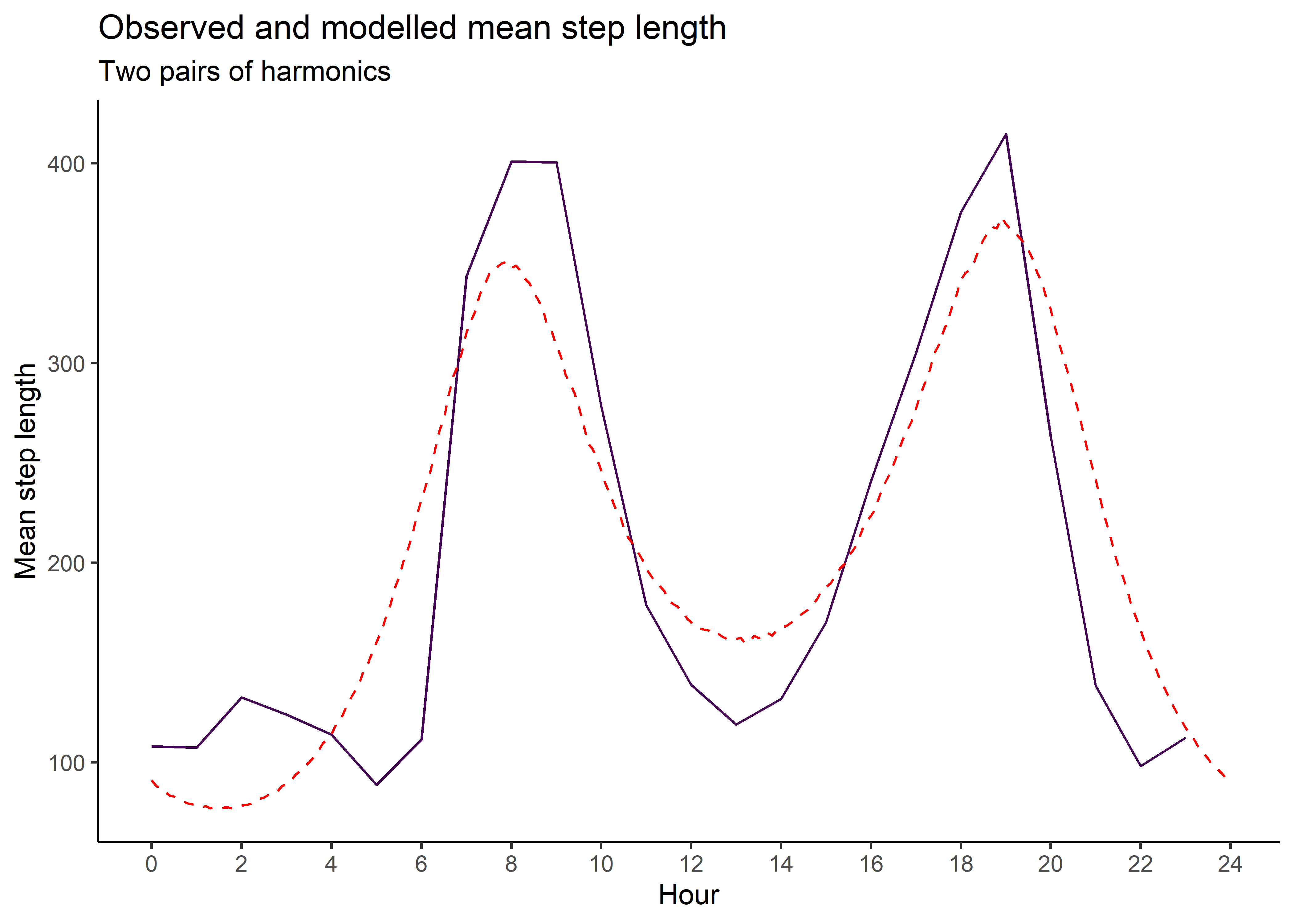
Code
median_sl_1p <- ggplot() +
  geom_path(data = movement_summary_buffalo,
            aes(x = hour, y = median_sl, colour = factor(id))) +
  geom_path(data = gamma_df_1p,
            aes(x = hour, y = median),
            colour = "red", linetype = "dashed") +
  scale_x_continuous("Hour", breaks = seq(0,24,2)) +
  scale_y_continuous("Median step length") +
  scale_colour_viridis_d("Buffalo") +
  ggtitle("Observed and modelled median step length",
          subtitle = "One pair of harmonics") +
  theme_classic() +
  theme(legend.position = "none")

median_sl_1p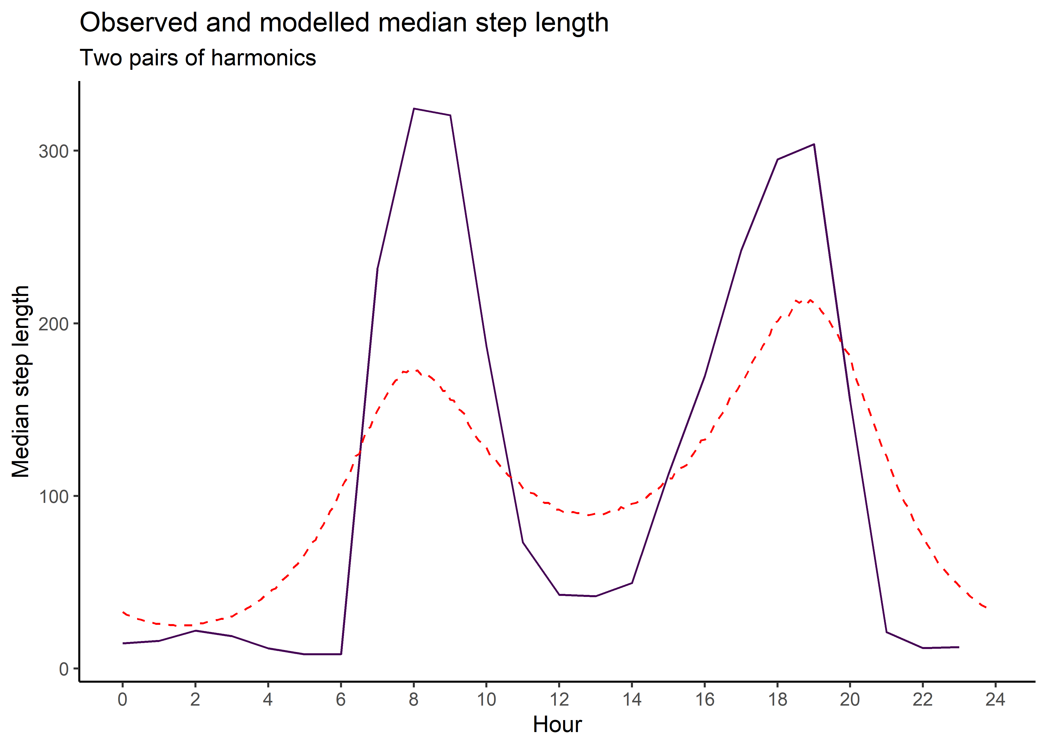
Code
Code
Code
Code
gamma_dist_list <- vector(mode = "list", length = nrow(hour_coefs_nat_df_2p))
gamma_mean <- c()
gamma_median <- c()
gamma_ratio <- c()

for(hour_no in 1:nrow(hour_coefs_nat_df_2p)) {

gamma_dist_list[[hour_no]] <- rgamma(n,
                                     shape = hour_coefs_nat_df_2p$shape[hour_no],
                                     scale = hour_coefs_nat_df_2p$scale[hour_no])

gamma_mean[hour_no] <- mean(gamma_dist_list[[hour_no]])
gamma_median[hour_no] <- median(gamma_dist_list[[hour_no]])
gamma_ratio[hour_no] <- gamma_mean[hour_no] / gamma_median[hour_no]

}

gamma_df_2p <- data.frame(model = "2p",
                          hour = hour_coefs_nat_df_2p$hour,
                          mean = gamma_mean,
                          median = gamma_median,
                          ratio = gamma_ratio)

mean_sl_2p <- ggplot() +
  geom_path(data = movement_summary_buffalo,
            aes(x = hour, y = mean_sl, colour = factor(id))) +
  geom_path(data = gamma_df_2p,
            aes(x = hour, y = mean),
            colour = "red", linetype = "dashed") +
  scale_x_continuous("Hour", breaks = seq(0,24,2)) +
  scale_y_continuous("Mean step length") +
  scale_colour_viridis_d("Buffalo") +
  ggtitle("Observed and modelled mean step length",
          subtitle = "Two pairs of harmonics") +
  theme_classic() +
  theme(legend.position = "none")

mean_sl_2p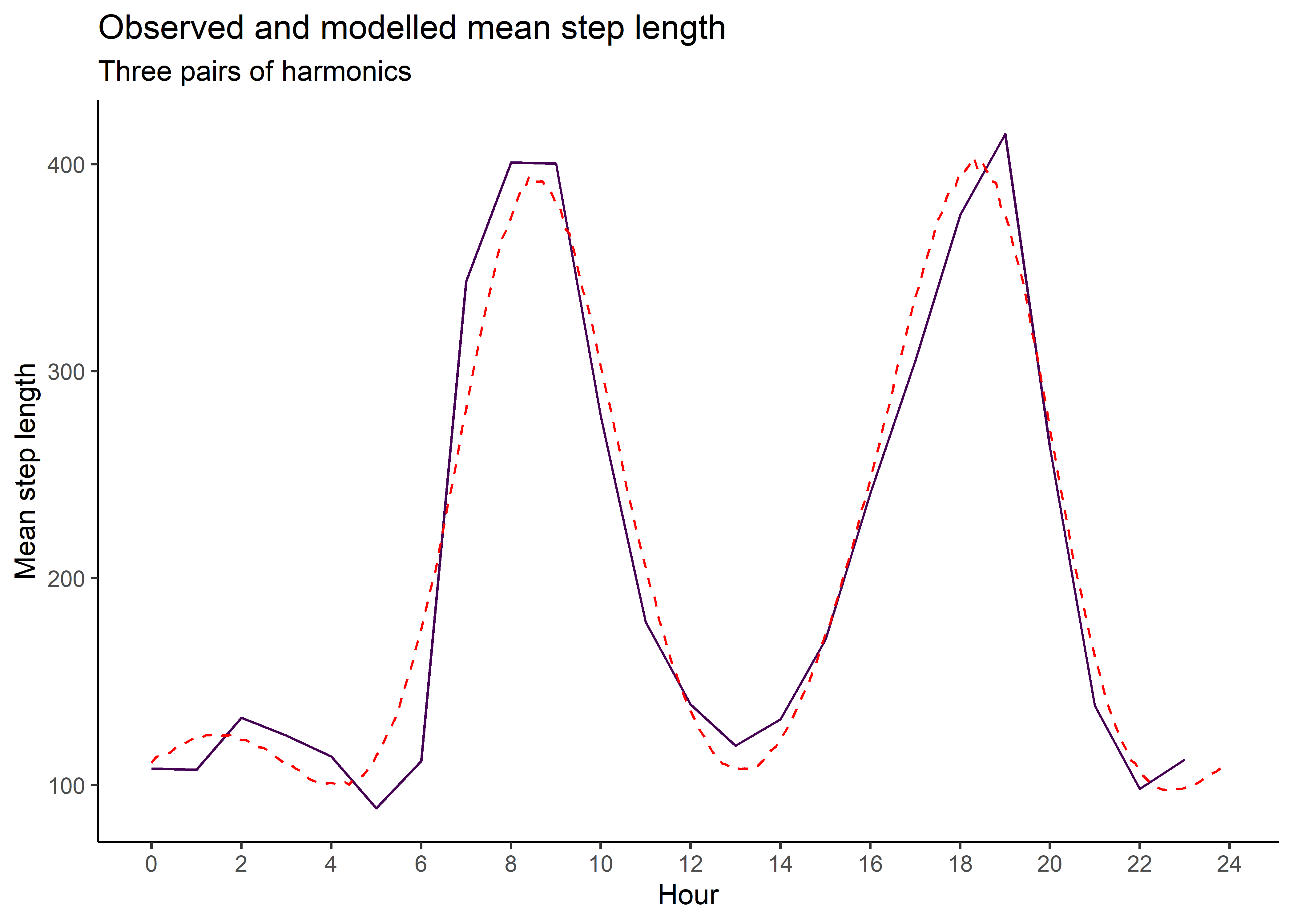
Code
median_sl_2p <- ggplot() +
  geom_path(data = movement_summary_buffalo,
            aes(x = hour, y = median_sl, colour = factor(id))) +
  geom_path(data = gamma_df_2p,
            aes(x = hour, y = median),
            colour = "red", linetype = "dashed") +
  scale_x_continuous("Hour", breaks = seq(0,24,2)) +
  scale_y_continuous("Median step length") +
  scale_colour_viridis_d("Buffalo") +
  ggtitle("Observed and modelled median step length",
          subtitle = "Two pairs of harmonics") +
  theme_classic() +
  theme(legend.position = "none")

median_sl_2p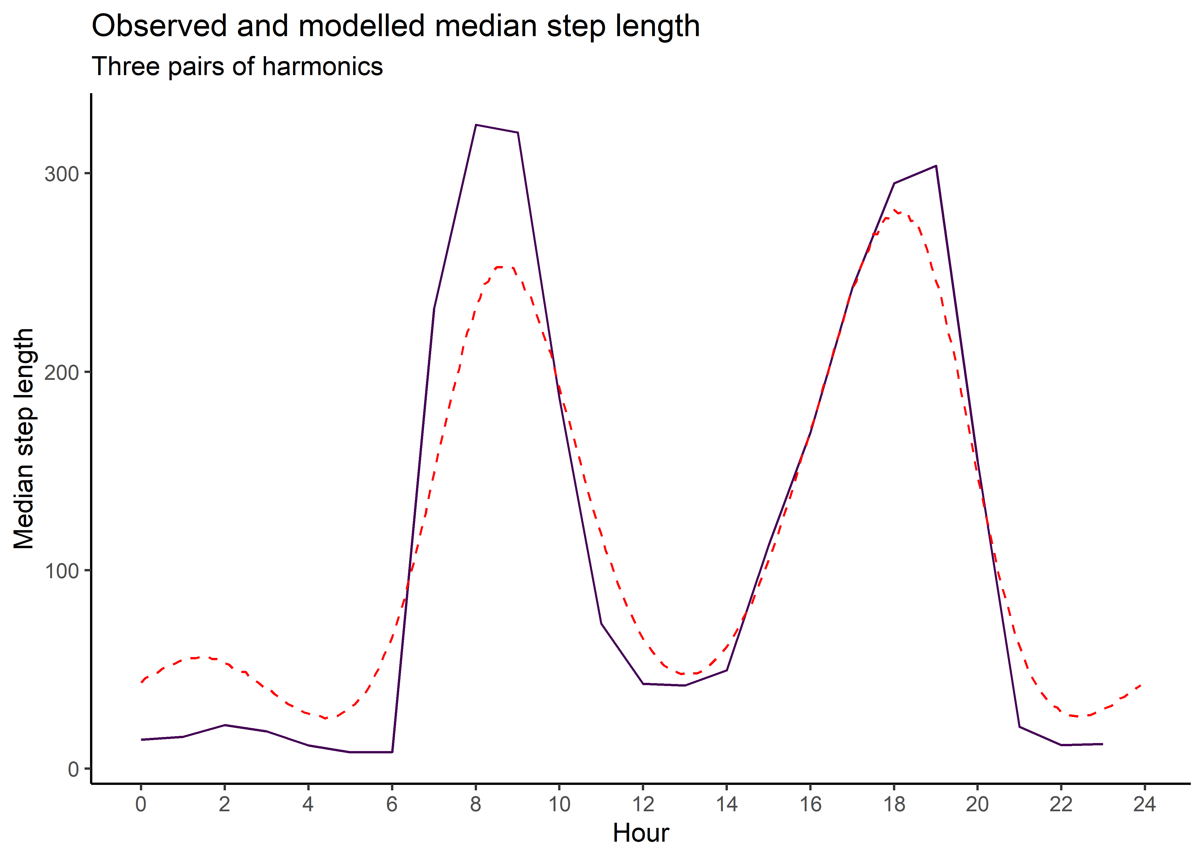
Code
Code
Code
Code
gamma_dist_list <- vector(mode = "list", length = nrow(hour_coefs_nat_df_3p))
gamma_mean <- c()
gamma_median <- c()
gamma_ratio <- c()

for(hour_no in 1:nrow(hour_coefs_nat_df_3p)) {

gamma_dist_list[[hour_no]] <- rgamma(n,
                                     shape = hour_coefs_nat_df_3p$shape[hour_no],
                                     scale = hour_coefs_nat_df_3p$scale[hour_no])

gamma_mean[hour_no] <- mean(gamma_dist_list[[hour_no]])
gamma_median[hour_no] <- median(gamma_dist_list[[hour_no]])
gamma_ratio[hour_no] <- gamma_mean[hour_no] / gamma_median[hour_no]

}

gamma_df_3p <- data.frame(model = "3p",
                          hour = hour_coefs_nat_df_3p$hour,
                          mean = gamma_mean,
                          median = gamma_median,
                          ratio = gamma_ratio)

mean_sl_3p <- ggplot() +
  geom_path(data = movement_summary_buffalo,
            aes(x = hour, y = mean_sl, colour = factor(id))) +
  geom_path(data = gamma_df_3p,
            aes(x = hour, y = mean),
            colour = "red", linetype = "dashed") +
  scale_x_continuous("Hour", breaks = seq(0,24,2)) +
  scale_y_continuous("Mean step length") +
  scale_colour_viridis_d("Buffalo") +
  ggtitle("Observed and modelled mean step length",
          subtitle = "Three pairs of harmonics") +
  theme_classic() +
  theme(legend.position = "none")

mean_sl_3p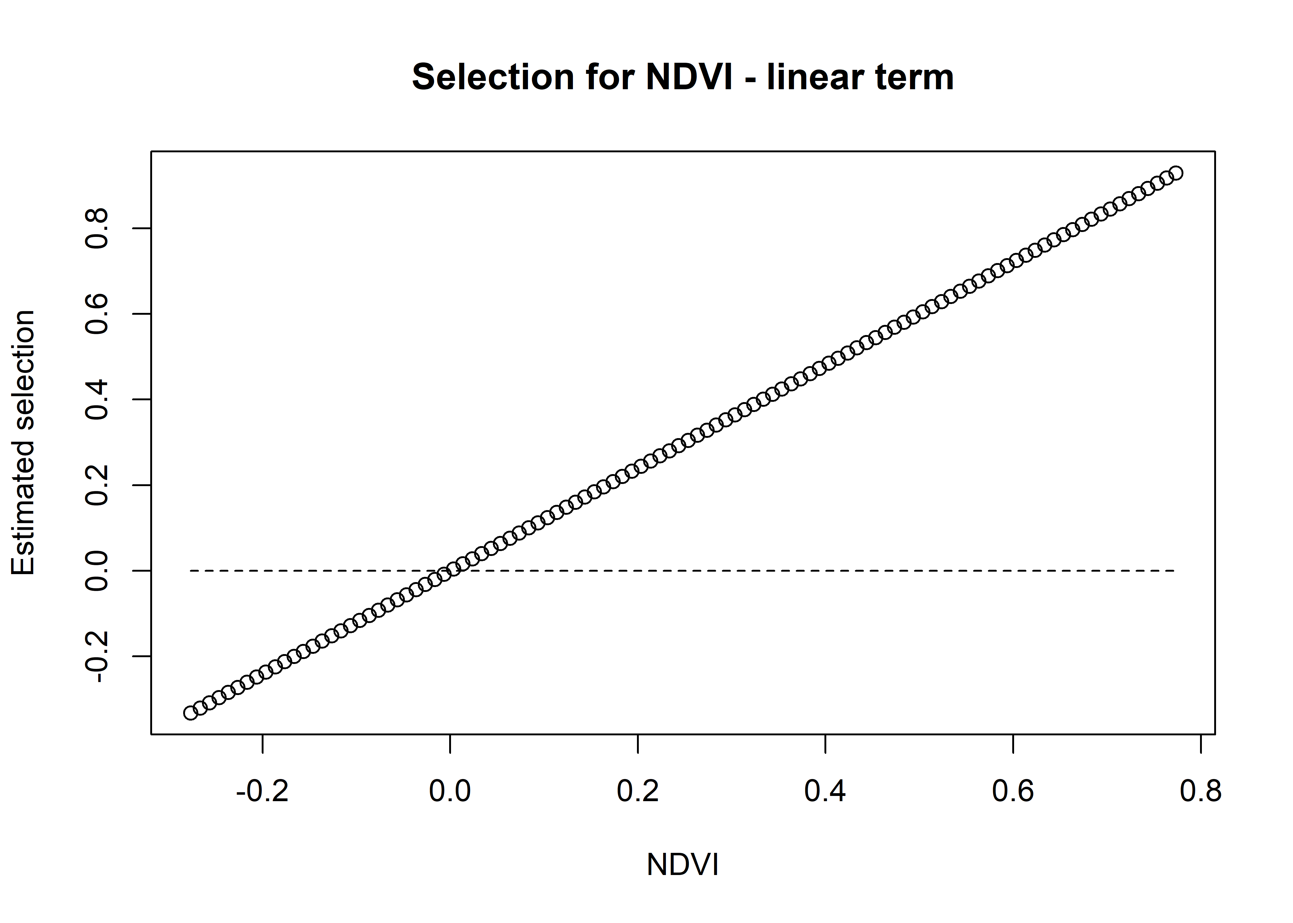
Code
median_sl_3p <- ggplot() +
  geom_path(data = movement_summary_buffalo,
            aes(x = hour, y = median_sl, colour = factor(id))) +
  geom_path(data = gamma_df_3p,
            aes(x = hour, y = median),
            colour = "red", linetype = "dashed") +
  scale_x_continuous("Hour", breaks = seq(0,24,2)) +
  scale_y_continuous("Median step length") +
  scale_colour_viridis_d("Buffalo") +
  ggtitle("Observed and modelled median step length",
          subtitle = "Three pairs of harmonics") +
  theme_classic() +
  theme(legend.position = "none")

median_sl_3p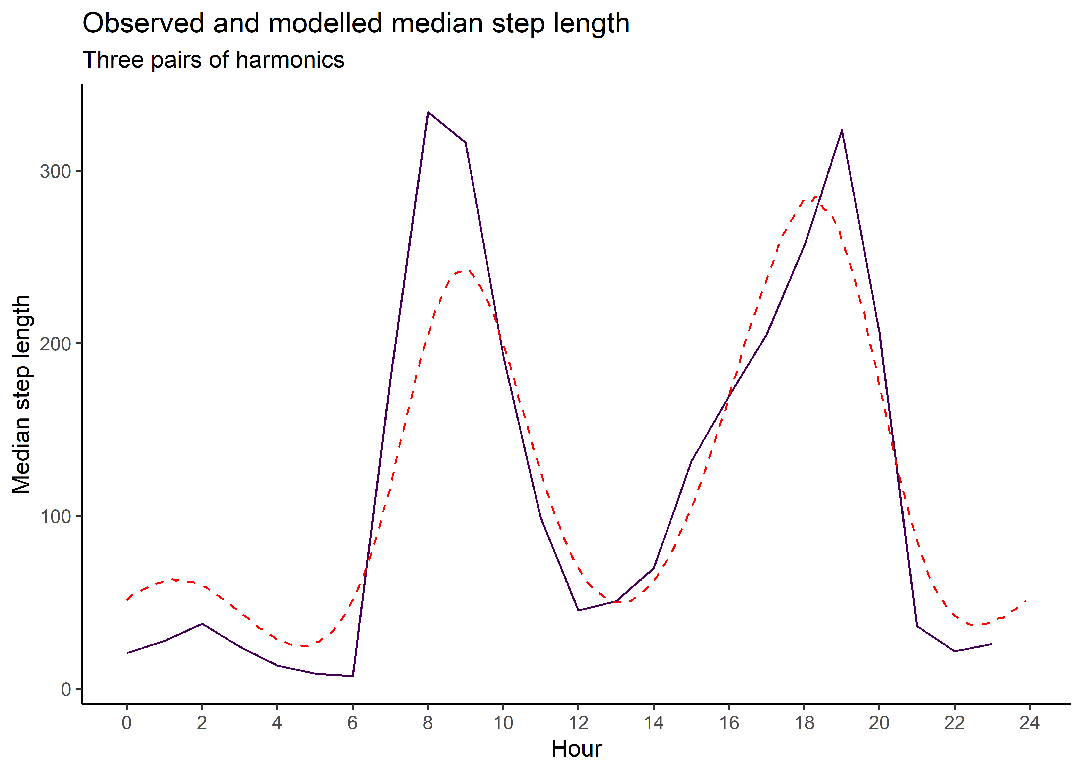
Code
Code
Code
Creating selection surfaces
As we have both quadratic and harmonic terms in the model, we can reconstruct a ‘selection surface’ to visualise how the animal’s respond to environmental features changes through time.
To illustrate, if we don’t have temporal dynamics (as is the case for this model), then we have a coefficient for the linear term and a coefficient for the quadratic term. Using these, we can plot the selection curve at the scale of the environmental variable (in this case NDVI).
Using the natural scale coefficients from the model:
Code
# first get a sequence of NDVI values,
# starting from the minimum observed in the data to the maximum
ndvi_min <- min(buffalo_data$ndvi_temporal, na.rm = TRUE)
ndvi_max <- max(buffalo_data$ndvi_temporal, na.rm = TRUE)
ndvi_seq <- seq(ndvi_min, ndvi_max, by = 0.01)

# take the coefficients from the model and calculation the selection value
# for every NDVI value in this sequence

# we can separate to the linear term
ndvi_linear_selection <- hour_coefs_nat_df_0p$ndvi[1] * ndvi_seq
plot(x = ndvi_seq, y = ndvi_linear_selection,
     main = "Selection for NDVI - linear term",
     xlab = "NDVI", ylab = "Estimated selection")
lines(ndvi_seq, rep(0,length(ndvi_seq)), lty = "dashed")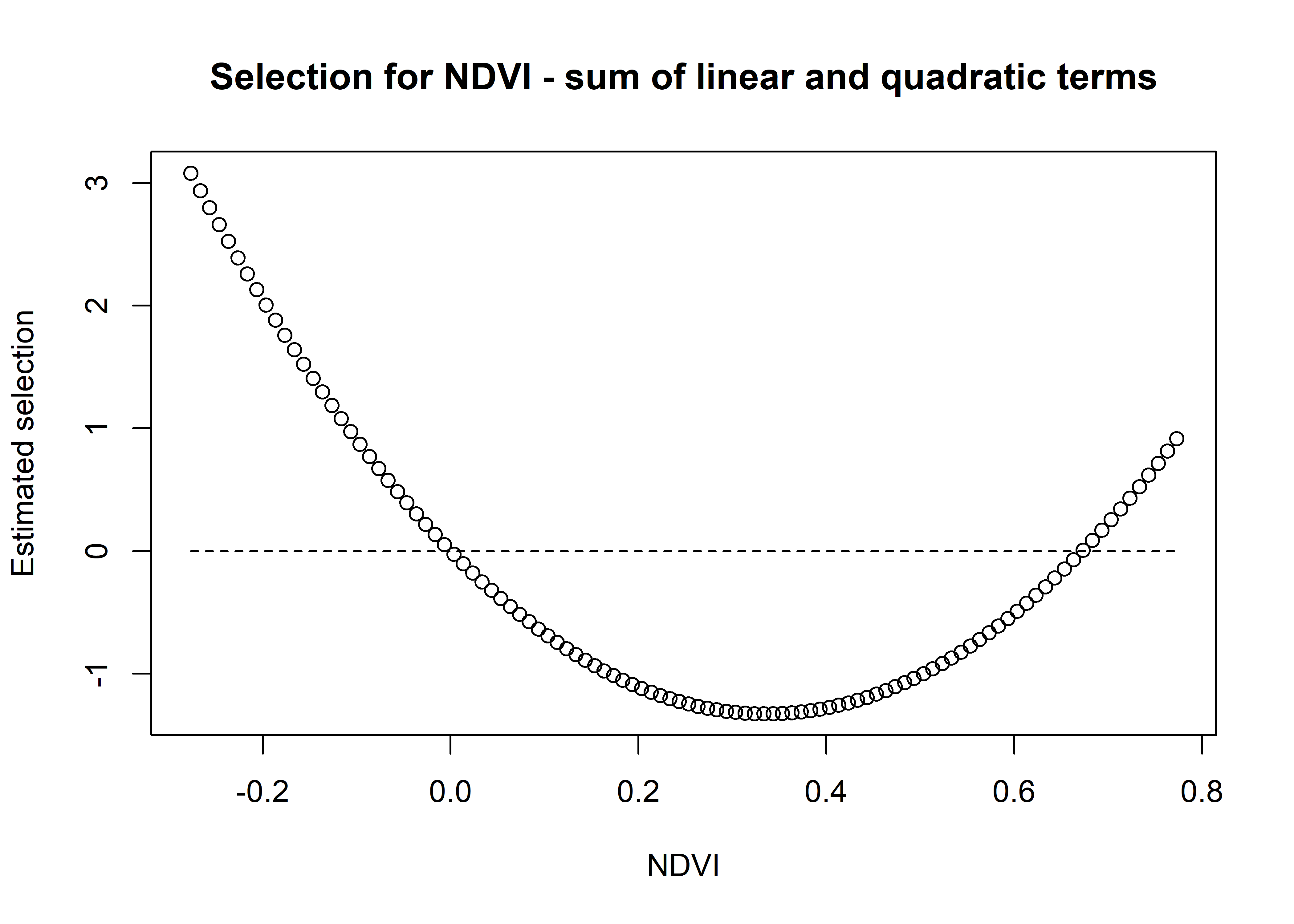
Code
Code
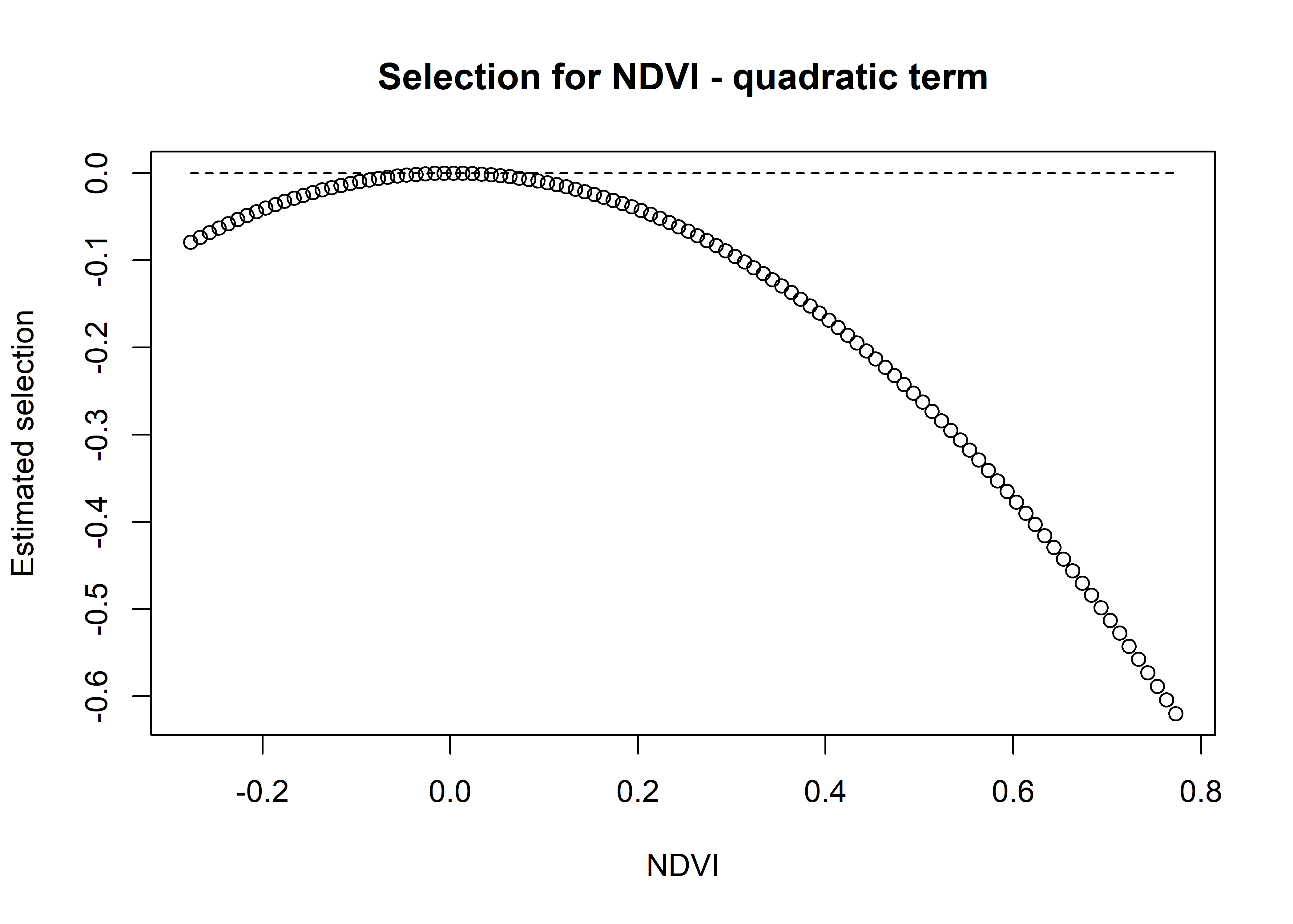
# and the sum of both
ndvi_sum_selection <- ndvi_linear_selection + ndvi_quadratic_selection
plot(x = ndvi_seq, y = ndvi_sum_selection,
     main = "Selection for NDVI - sum of linear and quadratic terms",
     xlab = "NDVI", ylab = "Estimated selection")
lines(ndvi_seq, rep(0,length(ndvi_seq)), lty = "dashed")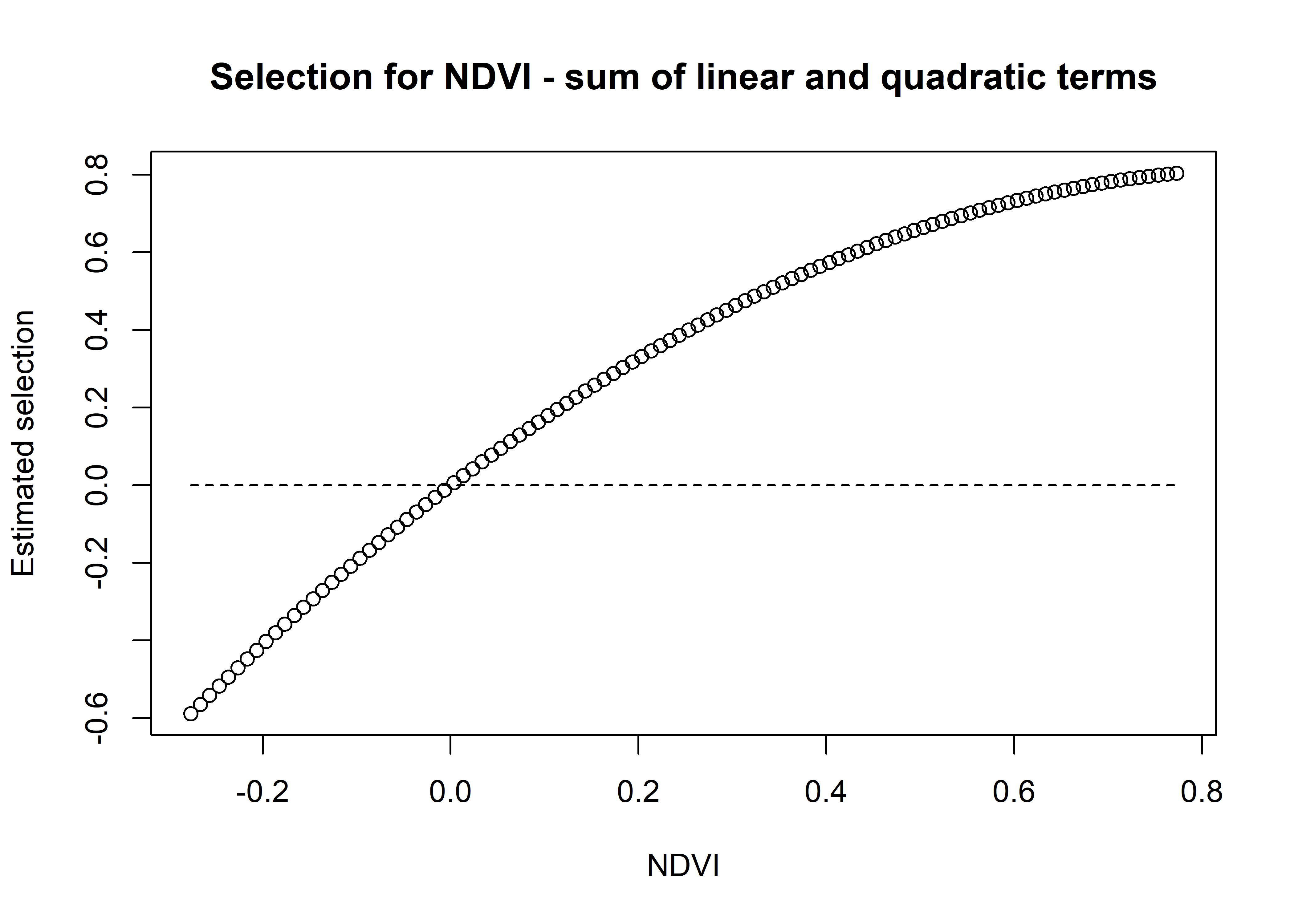
When there are no temporal dynamics, then this quadratic curve will be the same throughout the day, but when we have temporally dynamic coefficients for both the linear term and the quadratic term, then we will have a curves that vary continuously throughout the day, which we can visualise as a selection surface.
Here we illustrate for the model with 2 pairs of harmonic terms.
For brevity we won’t plot the linear and quadratic terms separately, but we can do so if needed.
First for Hour 3
Code
hour_no <- 3

# we can separate to the linear term
ndvi_linear_selection <-
  hour_coefs_nat_df_1p$ndvi[which(hour_coefs_nat_df_1p$hour == hour_no)] * ndvi_seq
# plot(x = ndvi_seq, y = ndvi_linear_selection,
#      main = "Selection for NDVI - linear term",
#      xlab = "NDVI", ylab = "Estimated selection")

# and the quadratic term
ndvi_quadratic_selection <-
  (hour_coefs_nat_df_1p$ndvi_2[which(hour_coefs_nat_df_1p$hour == hour_no)] * (ndvi_seq ^ 2))
# plot(x = ndvi_seq, y = ndvi_quadratic_selection,
#      main = "Selection for NDVI - quadratic term",
#      xlab = "NDVI", ylab = "Estimated selection")

# and the sum of both
ndvi_sum_selection <- ndvi_linear_selection + ndvi_quadratic_selection
plot(x = ndvi_seq, y = ndvi_sum_selection,
     main = "Selection for NDVI - sum of linear and quadratic terms",
     xlab = "NDVI", ylab = "Estimated selection")
lines(ndvi_seq, rep(0,length(ndvi_seq)), lty = "dashed")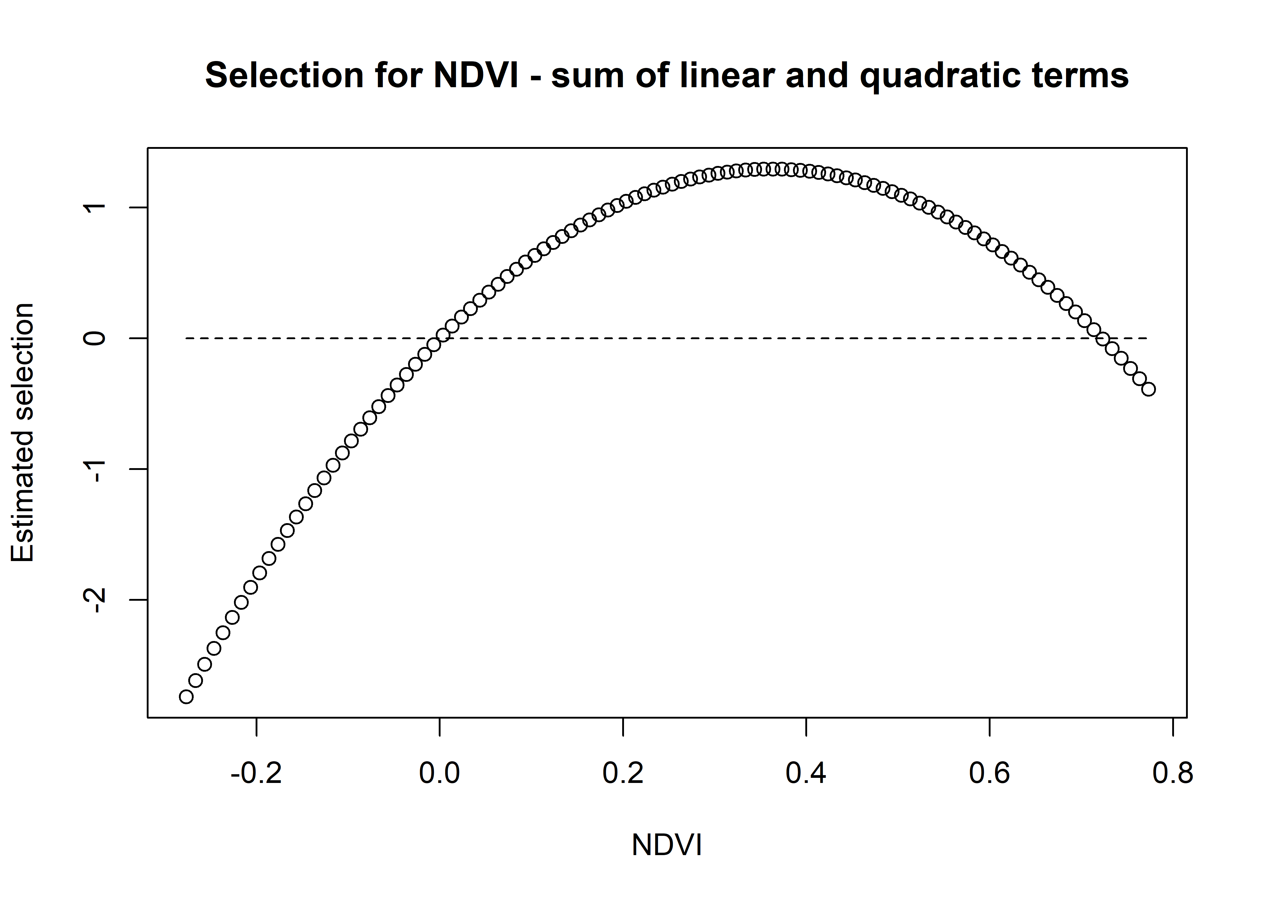
We can see that the coefficient at hour 3 shows highest selection for NDVI values slightly above 0.2, and the coefficient is mostly negative.
Secondly for Hour 12
Code
hour_no <- 12

# we can separate to the linear term
ndvi_linear_selection <-
  hour_coefs_nat_df_1p$ndvi[which(hour_coefs_nat_df_1p$hour == hour_no)] * ndvi_seq
# plot(x = ndvi_seq, y = ndvi_linear_selection,
#      main = "Selection for NDVI - linear term",
#      xlab = "NDVI", ylab = "Estimated selection")

# and the quadratic term
ndvi_quadratic_selection <-
  (hour_coefs_nat_df_1p$ndvi_2[which(hour_coefs_nat_df_1p$hour == hour_no)] * (ndvi_seq ^ 2))
# plot(x = ndvi_seq, y = ndvi_quadratic_selection,
#      main = "Selection for NDVI - quadratic term",
#      xlab = "NDVI", ylab = "Estimated selection")

# and the sum of both
ndvi_sum_selection <- ndvi_linear_selection + ndvi_quadratic_selection
plot(x = ndvi_seq, y = ndvi_sum_selection,
     main = "Selection for NDVI - sum of linear and quadratic terms",
     xlab = "NDVI", ylab = "Estimated selection")
lines(ndvi_seq, rep(0,length(ndvi_seq)), lty = "dashed")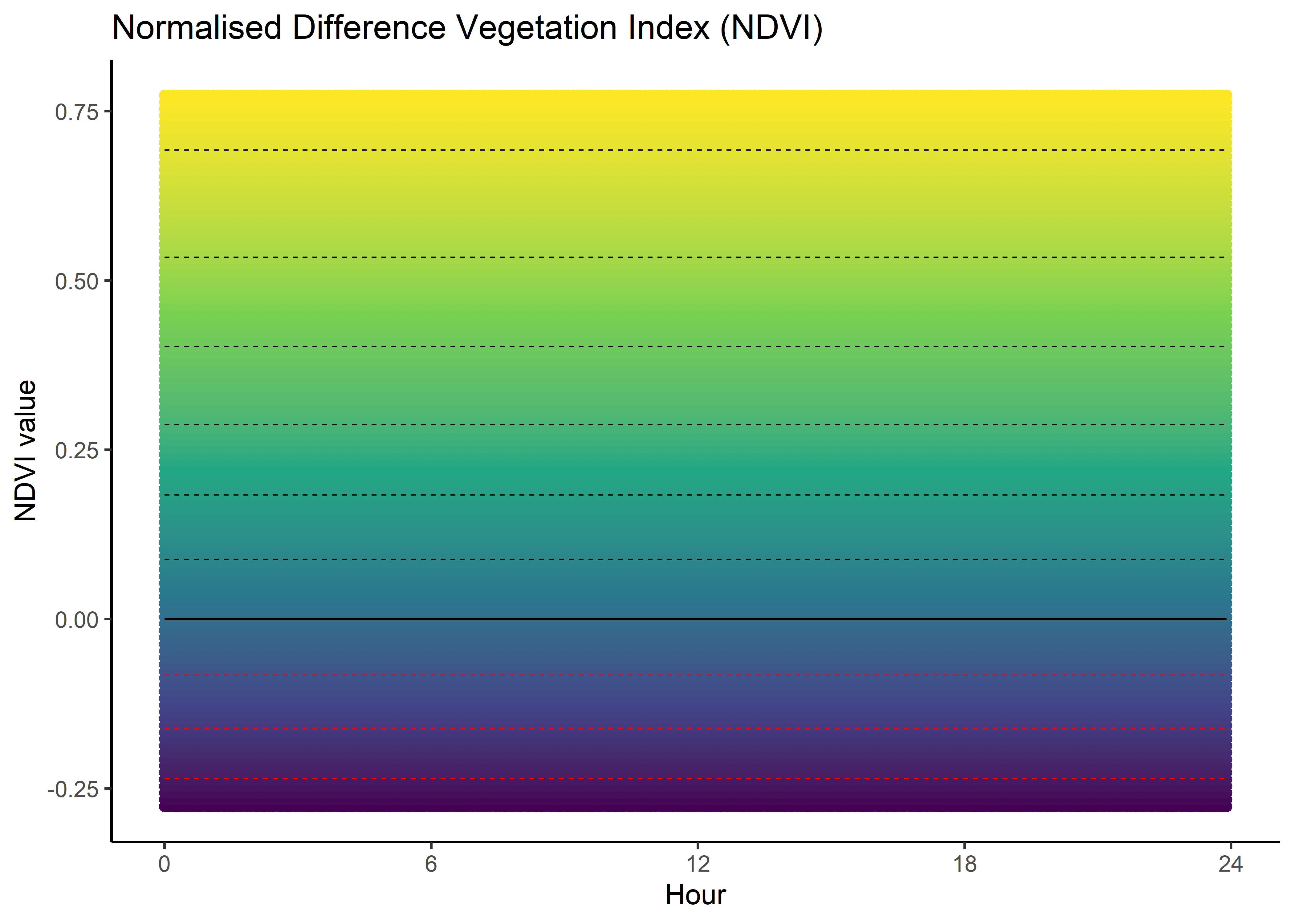
Whereas for hour 12, the coefficient shows highest selection for NDVI values slightly above 0.4, and the coefficient is positive for NDVI values above 0.
We can imagine viewing these plots for every hour of the day, where each hour has a different quadratic curve, but this would be a lot of plots. We can also see it as a 3D surface, where the x-axis is the hour of the day, the y-axis is the NDVI value, and the z-axis (colour) is the coefficient value.
We simply index over the linear and quadratic terms and calculate the coefficient values at every time point.
NDVI selection surface
Code
ndvi_min <- min(buffalo_data$ndvi_temporal, na.rm = TRUE)
ndvi_max <- max(buffalo_data$ndvi_temporal, na.rm = TRUE)
ndvi_seq <- seq(ndvi_min, ndvi_max, by = 0.01)

# Create empty data frame
ndvi_fresponse_df <- data.frame(matrix(ncol = nrow(hour_coefs_nat_df_0p),
                                       nrow = length(ndvi_seq)))

# loop over each time increment, calculating the selection values for each NDVI value
# and storing each time increment as a column in a dataframe that we can use for plotting
for(i in 1:nrow(hour_coefs_nat_df_0p)) {
  # Assign the vector as a column to the dataframe
  ndvi_fresponse_df[,i] <- (hour_coefs_nat_df_0p$ndvi[i] * ndvi_seq) +
    (hour_coefs_nat_df_0p$ndvi_2[i] * (ndvi_seq ^ 2))
}

ndvi_fresponse_df <- data.frame(ndvi_seq, ndvi_fresponse_df)
colnames(ndvi_fresponse_df) <- c("ndvi", hour)
ndvi_fresponse_long <- pivot_longer(ndvi_fresponse_df,
                                    cols = !1, names_to = "hour")

ndvi_contour_max <- max(ndvi_fresponse_long$value) # 0.7890195
ndvi_contour_min <- min(ndvi_fresponse_long$value) # -0.7945691
ndvi_contour_increment <- (ndvi_contour_max-ndvi_contour_min)/10

ndvi_quad_0p <- ggplot(data = ndvi_fresponse_long,
                       aes(x = as.numeric(hour), y = ndvi)) +
  geom_point(aes(colour = value)) +
  geom_contour(aes(z = value),
               breaks = seq(ndvi_contour_increment,
                            ndvi_contour_max,
                            ndvi_contour_increment),
               colour = "black", linewidth = 0.25, linetype = "dashed") +
  geom_contour(aes(z = value),
               breaks = seq(-ndvi_contour_increment,
                            ndvi_contour_min,
                            -ndvi_contour_increment),
               colour = "red", linewidth = 0.25, linetype = "dashed") +
  geom_contour(aes(z = value), breaks = 0, colour = "black", linewidth = 0.5) +
  scale_x_continuous("Hour", breaks = seq(0,24,6)) +
  scale_y_continuous("NDVI value", breaks = seq(-1, 1, 0.25)) +
  scale_colour_viridis_c("Selection") +
  ggtitle("Normalised Difference Vegetation Index (NDVI)") +
  theme_classic() +
  theme(legend.position = "none")

ndvi_quad_0p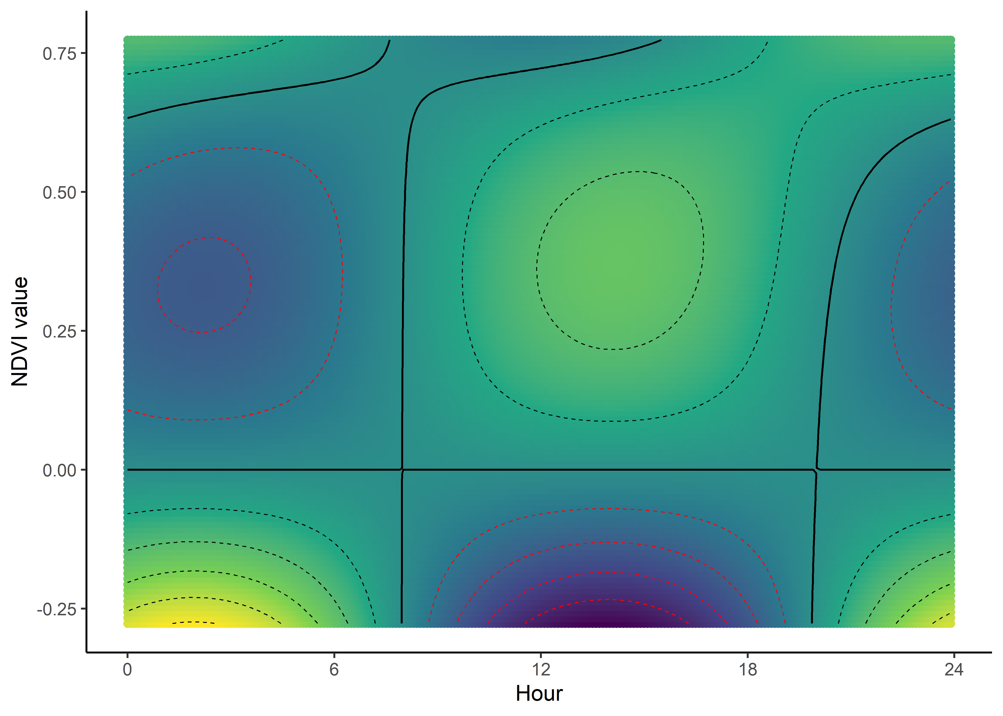
Code
ndvi_min <- min(buffalo_data$ndvi_temporal, na.rm = TRUE)
ndvi_max <- max(buffalo_data$ndvi_temporal, na.rm = TRUE)
ndvi_seq <- seq(ndvi_min, ndvi_max, by = 0.01)

# Create empty data frame
ndvi_fresponse_df <- data.frame(matrix(ncol = nrow(hour_coefs_nat_df_1p),
                                       nrow = length(ndvi_seq)))

for(i in 1:nrow(hour_coefs_nat_df_1p)) {
  # Assign the vector as a column to the dataframe
  ndvi_fresponse_df[,i] <- (hour_coefs_nat_df_1p$ndvi[i] * ndvi_seq) +
    (hour_coefs_nat_df_1p$ndvi_2[i] * (ndvi_seq ^ 2))
}

ndvi_fresponse_df <- data.frame(ndvi_seq, ndvi_fresponse_df)
colnames(ndvi_fresponse_df) <- c("ndvi", hour)
ndvi_fresponse_long <- pivot_longer(ndvi_fresponse_df, cols = !1, names_to = "hour")

ndvi_contour_max <- max(ndvi_fresponse_long$value) # 0.7890195
ndvi_contour_min <- min(ndvi_fresponse_long$value) # -0.7945691
ndvi_contour_increment <- (ndvi_contour_max-ndvi_contour_min)/10

ndvi_quad_1p <- ggplot(data = ndvi_fresponse_long,
                       aes(x = as.numeric(hour), y = ndvi)) +
  geom_point(aes(colour = value)) + # colour = "white"
  geom_contour(aes(z = value),
               breaks = seq(ndvi_contour_increment,
                            ndvi_contour_max,
                            ndvi_contour_increment),
               colour = "black", linewidth = 0.25, linetype = "dashed") +
  geom_contour(aes(z = value),
               breaks = seq(-ndvi_contour_increment,
                            ndvi_contour_min,
                            -ndvi_contour_increment),
               colour = "red", linewidth = 0.25, linetype = "dashed") +
  geom_contour(aes(z = value), breaks = 0, colour = "black", linewidth = 0.5) +
  scale_x_continuous("Hour", breaks = seq(0,24,6)) +
  scale_y_continuous("NDVI value", breaks = seq(-1, 1, 0.25)) +
  scale_colour_viridis_c("Selection") +
  # ggtitle("Normalised Difference Vegetation Index (NDVI)") +
  theme_classic() +
  theme(legend.position = "none")

ndvi_quad_1p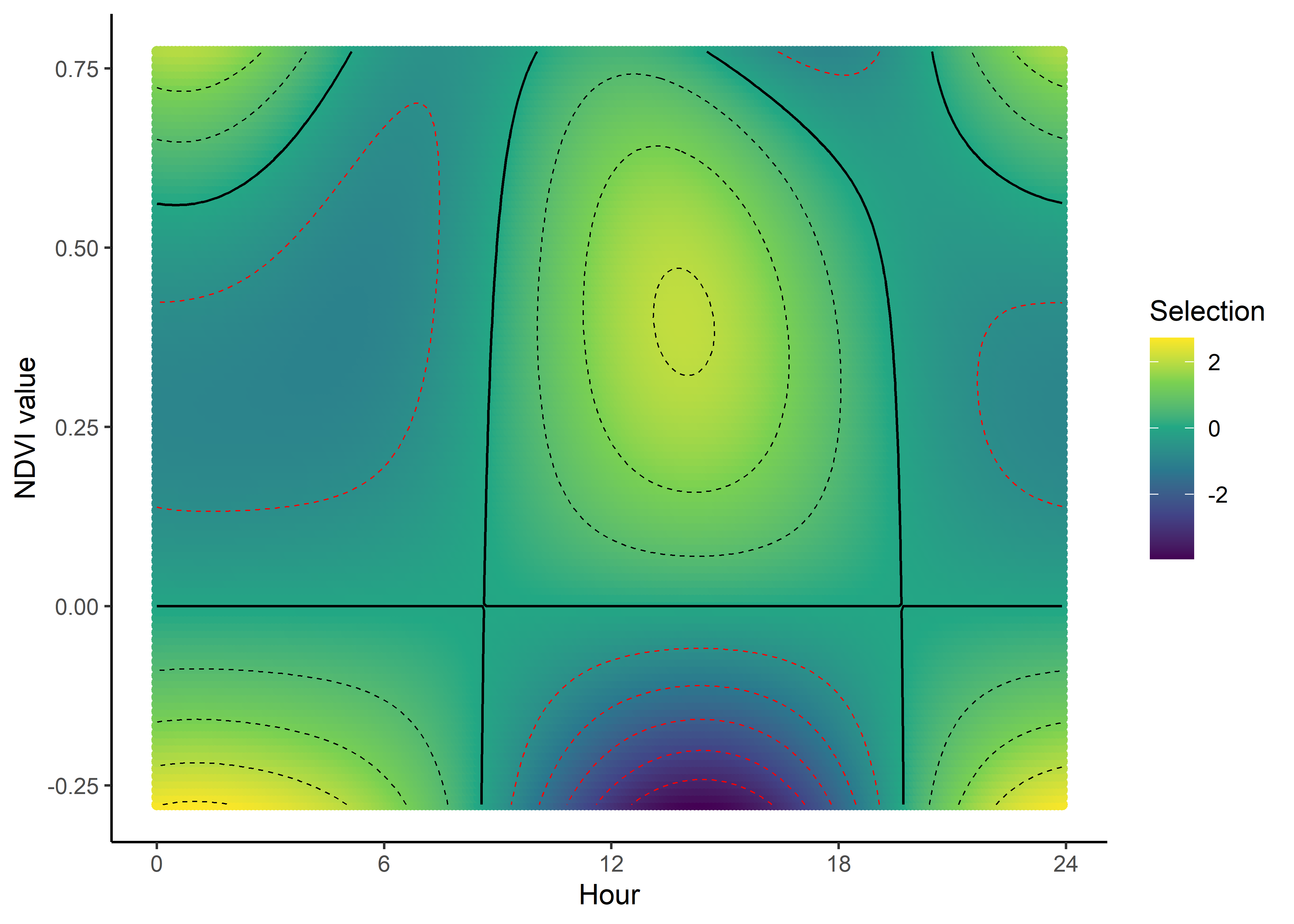
Code
ndvi_min <- min(buffalo_data$ndvi_temporal, na.rm = TRUE)
ndvi_max <- max(buffalo_data$ndvi_temporal, na.rm = TRUE)
ndvi_seq <- seq(ndvi_min, ndvi_max, by = 0.01)

# Create empty data frame
ndvi_fresponse_df <- data.frame(matrix(ncol = nrow(hour_coefs_nat_df_2p),
                                       nrow = length(ndvi_seq)))

for(i in 1:nrow(hour_coefs_nat_df_2p)) {
  # Assign the vector as a column to the dataframe
  ndvi_fresponse_df[,i] <- (hour_coefs_nat_df_2p$ndvi[i] * ndvi_seq) +
    (hour_coefs_nat_df_2p$ndvi_2[i] * (ndvi_seq ^ 2))
}

ndvi_fresponse_df <- data.frame(ndvi_seq, ndvi_fresponse_df)
colnames(ndvi_fresponse_df) <- c("ndvi", hour)
ndvi_fresponse_long <- pivot_longer(ndvi_fresponse_df, cols = !1,
                                    names_to = "hour")

ndvi_contour_max <- max(ndvi_fresponse_long$value) # 0.7890195
ndvi_contour_min <- min(ndvi_fresponse_long$value) # -0.7945691
ndvi_contour_increment <- (ndvi_contour_max-ndvi_contour_min)/10

ndvi_quad_2p <- ggplot(data = ndvi_fresponse_long,
                       aes(x = as.numeric(hour), y = ndvi)) +
  geom_point(aes(colour = value)) + # colour = "white"
  geom_contour(aes(z = value),
               breaks = seq(ndvi_contour_increment,
                            ndvi_contour_max,
                            ndvi_contour_increment),
               colour = "black", linewidth = 0.25, linetype = "dashed") +
  geom_contour(aes(z = value),
               breaks = seq(-ndvi_contour_increment,
                            ndvi_contour_min,
                            -ndvi_contour_increment),
               colour = "red", linewidth = 0.25, linetype = "dashed") +
  geom_contour(aes(z = value), breaks = 0, colour = "black", linewidth = 0.5) +
  scale_x_continuous("Hour", breaks = seq(0,24,6)) +
  scale_y_continuous("NDVI value", breaks = seq(-1, 1, 0.25)) +
  scale_colour_viridis_c("Selection") +
  # ggtitle("Normalised Difference Vegetation Index (NDVI)") +
  theme_classic() +
  theme(legend.position = "right")

ndvi_quad_2p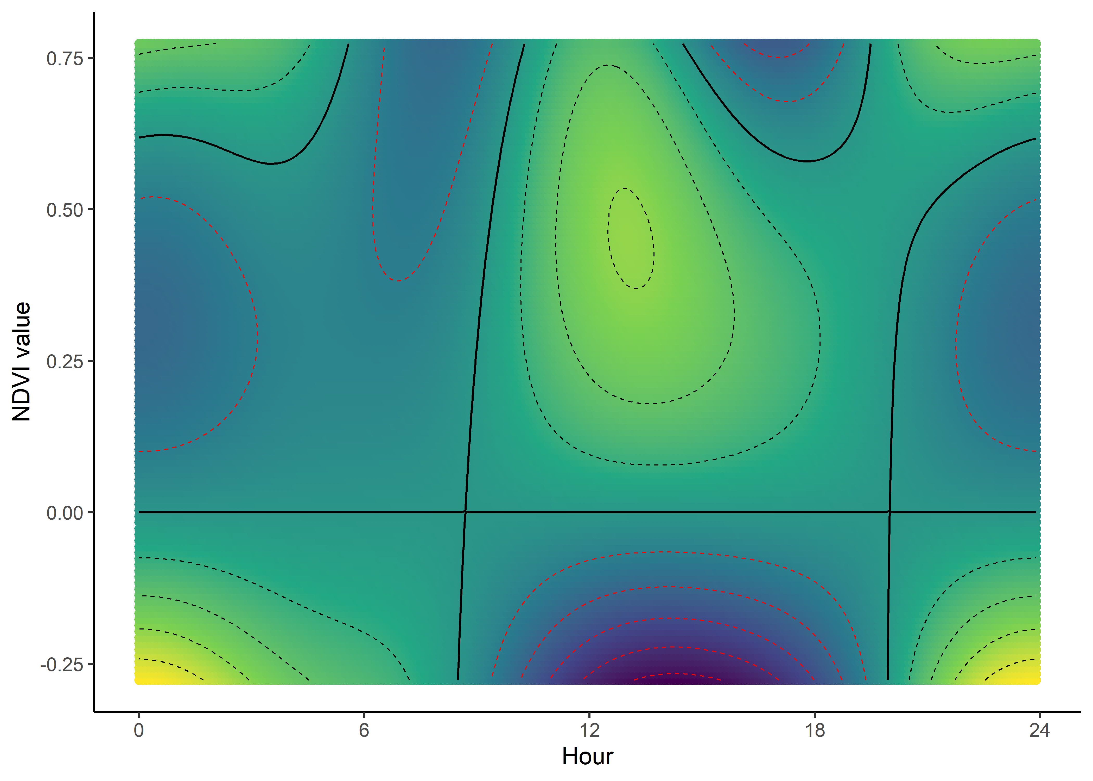
Code
ndvi_min <- min(buffalo_data$ndvi_temporal, na.rm = TRUE)
ndvi_max <- max(buffalo_data$ndvi_temporal, na.rm = TRUE)
ndvi_seq <- seq(ndvi_min, ndvi_max, by = 0.01)

# Create empty data frame
ndvi_fresponse_df <- data.frame(matrix(ncol = nrow(hour_coefs_nat_df_3p),
                                       nrow = length(ndvi_seq)))

for(i in 1:nrow(hour_coefs_nat_df_3p)) {
  # Assign the vector as a column to the dataframe
  ndvi_fresponse_df[,i] <- (hour_coefs_nat_df_3p$ndvi[i] * ndvi_seq) +
    (hour_coefs_nat_df_3p$ndvi_2[i] * (ndvi_seq ^ 2))
}

ndvi_fresponse_df <- data.frame(ndvi_seq, ndvi_fresponse_df)
colnames(ndvi_fresponse_df) <- c("ndvi", hour)
ndvi_fresponse_long <- pivot_longer(ndvi_fresponse_df, cols = !1,
                                    names_to = "hour")

ndvi_contour_max <- max(ndvi_fresponse_long$value) # 0.7890195
ndvi_contour_min <- min(ndvi_fresponse_long$value) # -0.7945691
ndvi_contour_increment <- (ndvi_contour_max-ndvi_contour_min)/10

ndvi_quad_3p <- ggplot(data = ndvi_fresponse_long,
                       aes(x = as.numeric(hour), y = ndvi)) +
  geom_point(aes(colour = value)) + # colour = "white"
  geom_contour(aes(z = value),
               breaks = seq(ndvi_contour_increment,
                            ndvi_contour_max,
                            ndvi_contour_increment),
               colour = "black", linewidth = 0.25, linetype = "dashed") +
  geom_contour(aes(z = value),
               breaks = seq(-ndvi_contour_increment,
                            ndvi_contour_min,
                            -ndvi_contour_increment),
               colour = "red", linewidth = 0.25, linetype = "dashed") +
  geom_contour(aes(z = value), breaks = 0, colour = "black", linewidth = 0.5) +
  scale_x_continuous("Hour", breaks = seq(0,24,6)) +
  scale_y_continuous("NDVI value", breaks = seq(-1, 1, 0.25)) +
  scale_colour_viridis_c("Selection") +
  # ggtitle("Normalised Difference Vegetation Index (NDVI)") +
  theme_classic() +
  theme(legend.position = "none")

ndvi_quad_3p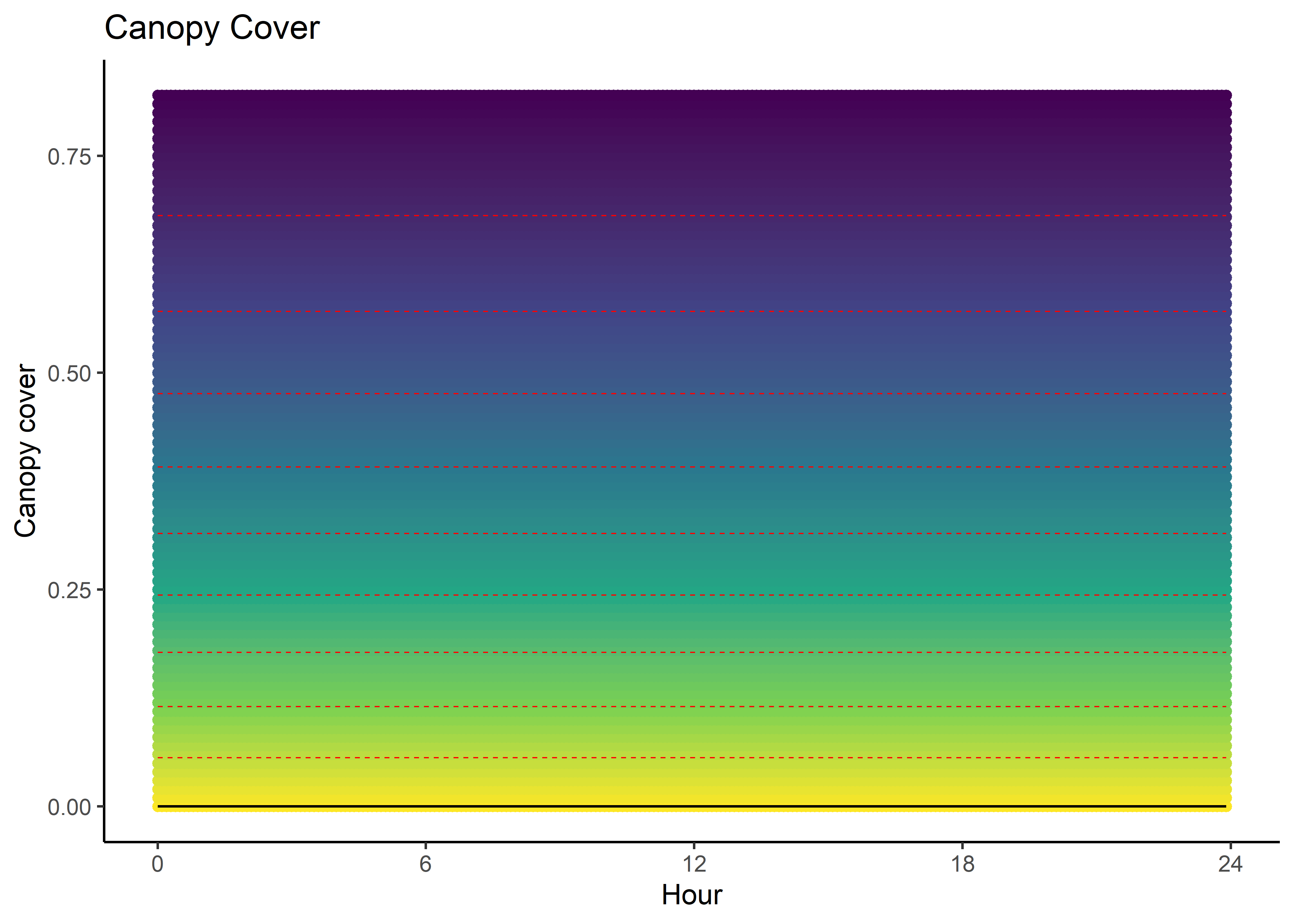
Canopy cover selection surface
Code
canopy_min <- min(buffalo_data$canopy_01, na.rm = TRUE)
canopy_max <- max(buffalo_data$canopy_01, na.rm = TRUE)
canopy_seq <- seq(canopy_min, canopy_max, by = 0.01)

# Create empty data frame
canopy_fresponse_df <- data.frame(matrix(ncol = nrow(hour_coefs_nat_df_0p),
                                         nrow = length(canopy_seq)))

for(i in 1:nrow(hour_coefs_nat_df_0p)) {
  # Assign the vector as a column to the dataframe
  canopy_fresponse_df[,i] <- (hour_coefs_nat_df_0p$canopy[i] * canopy_seq) +
    (hour_coefs_nat_df_0p$canopy_2[i] * (canopy_seq ^ 2))
}

canopy_fresponse_df <- data.frame(canopy_seq, canopy_fresponse_df)
colnames(canopy_fresponse_df) <- c("canopy", hour)
canopy_fresponse_long <- pivot_longer(canopy_fresponse_df,
                                      cols = !1,
                                      names_to = "hour")

canopy_contour_min <- min(canopy_fresponse_long$value) # 0
canopy_contour_max <- max(canopy_fresponse_long$value) # 2.181749
canopy_contour_increment <- (canopy_contour_max-canopy_contour_min)/10

canopy_quad_0p <- ggplot(data = canopy_fresponse_long, aes(x = as.numeric(hour),
                                                           y = canopy)) +
  geom_point(aes(colour = value)) +
  geom_contour(aes(z = value),
               breaks = seq(canopy_contour_increment, canopy_contour_max,
                            -canopy_contour_increment),
               colour = "black", linewidth = 0.25, linetype = "dashed") +
  geom_contour(aes(z = value),
  breaks = seq(-canopy_contour_increment, canopy_contour_min,
               -canopy_contour_increment),
               colour = "red", linewidth = 0.25, linetype = "dashed") +
  geom_contour(aes(z = value), breaks = 0, colour = "black", linewidth = 0.5) +
  scale_x_continuous("Hour", breaks = seq(0,24,6)) +
  scale_y_continuous("Canopy cover", breaks = seq(0, 1, 0.25)) +
  scale_colour_viridis_c("Selection") +
  ggtitle("Canopy Cover") +
  theme_classic() +
  theme(legend.position = "none")

canopy_quad_0p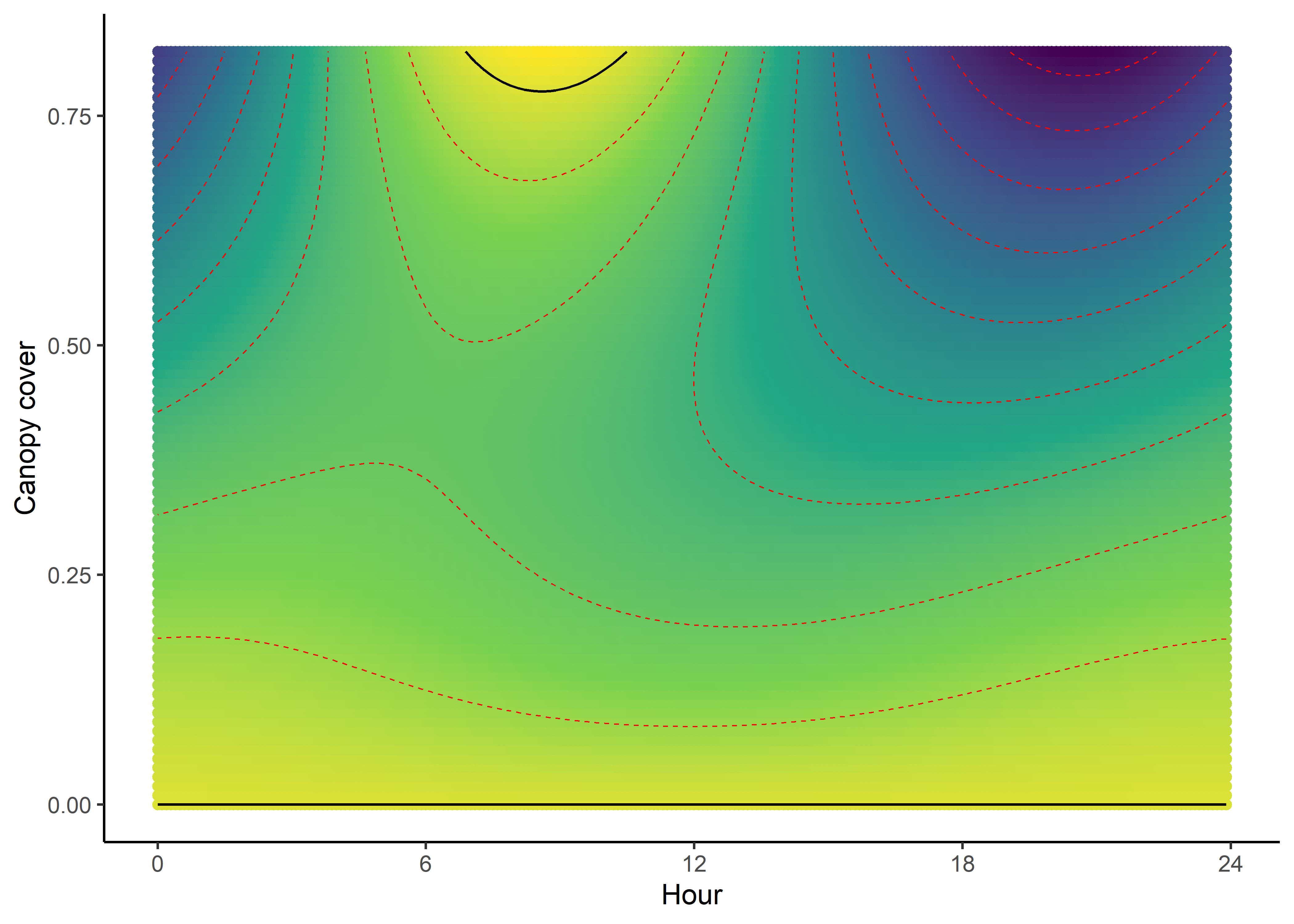
Code
canopy_min <- min(buffalo_data$canopy_01, na.rm = TRUE)
canopy_max <- max(buffalo_data$canopy_01, na.rm = TRUE)
canopy_seq <- seq(canopy_min, canopy_max, by = 0.01)

# Create empty data frame
canopy_fresponse_df <- data.frame(matrix(ncol = nrow(hour_coefs_nat_df_1p),
                                         nrow = length(canopy_seq)))

for(i in 1:nrow(hour_coefs_nat_df_1p)) {
  # Assign the vector as a column to the dataframe
  canopy_fresponse_df[,i] <- (hour_coefs_nat_df_1p$canopy[i] * canopy_seq) +
    (hour_coefs_nat_df_1p$canopy_2[i] * (canopy_seq ^ 2))
}

canopy_fresponse_df <- data.frame(canopy_seq, canopy_fresponse_df)
colnames(canopy_fresponse_df) <- c("canopy", hour)
canopy_fresponse_long <- pivot_longer(canopy_fresponse_df, cols = !1,
                                      names_to = "hour")

canopy_contour_min <- min(canopy_fresponse_long$value) # 0
canopy_contour_max <- max(canopy_fresponse_long$value) # 2.181749
canopy_contour_increment <- (canopy_contour_max-canopy_contour_min)/10

canopy_quad_1p <- ggplot(data = canopy_fresponse_long,
                         aes(x = as.numeric(hour), y = canopy)) +
  geom_point(aes(colour = value)) +
  geom_contour(aes(z = value),
               breaks = seq(canopy_contour_increment,
                            canopy_contour_max,
                            canopy_contour_increment),
               colour = "black", linewidth = 0.25, linetype = "dashed") +
  geom_contour(aes(z = value),
               breaks = seq(-canopy_contour_increment,
                            canopy_contour_min,
                            -canopy_contour_increment),
               colour = "red", linewidth = 0.25, linetype = "dashed") +
  geom_contour(aes(z = value), breaks = 0, colour = "black", linewidth = 0.5) +
  scale_x_continuous("Hour", breaks = seq(0,24,6)) +
  scale_y_continuous("Canopy cover", breaks = seq(0, 1, 0.25)) +
  scale_colour_viridis_c("Selection") +
  # ggtitle("Canopy Cover") +
  theme_classic() +
  theme(legend.position = "none")

canopy_quad_1p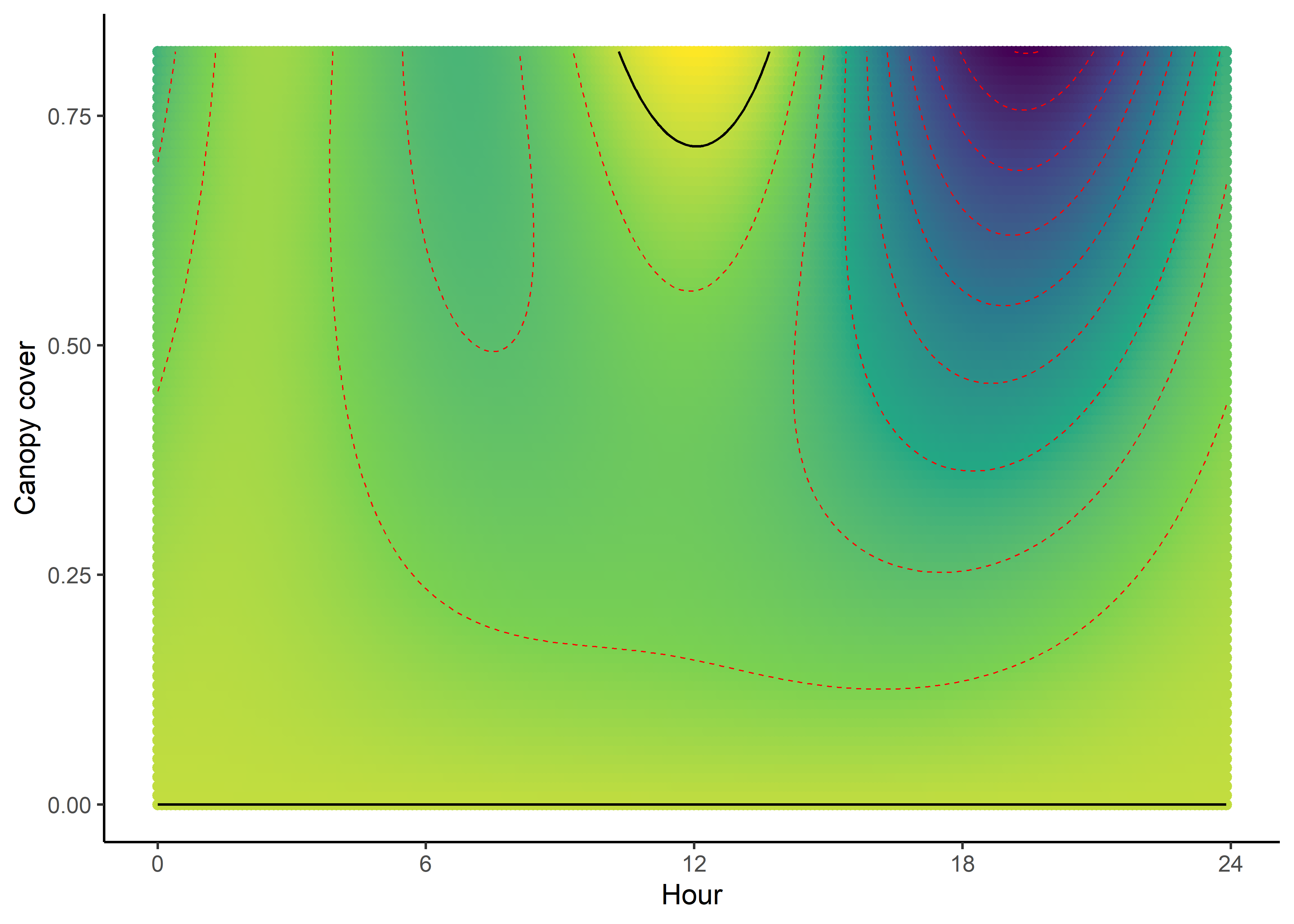
Code
canopy_min <- min(buffalo_data$canopy_01, na.rm = TRUE)
canopy_max <- max(buffalo_data$canopy_01, na.rm = TRUE)
canopy_seq <- seq(canopy_min, canopy_max, by = 0.01)

# Create empty data frame
canopy_fresponse_df <- data.frame(matrix(ncol = nrow(hour_coefs_nat_df_2p),
                                         nrow = length(canopy_seq)))

for(i in 1:nrow(hour_coefs_nat_df_2p)) {
  # Assign the vector as a column to the dataframe
  canopy_fresponse_df[,i] <- (hour_coefs_nat_df_2p$canopy[i] * canopy_seq) +
    (hour_coefs_nat_df_2p$canopy_2[i] * (canopy_seq ^ 2))
}

canopy_fresponse_df <- data.frame(canopy_seq, canopy_fresponse_df)
colnames(canopy_fresponse_df) <- c("canopy", hour)
canopy_fresponse_long <- pivot_longer(canopy_fresponse_df, cols = !1,
                                      names_to = "hour")

canopy_contour_min <- min(canopy_fresponse_long$value) # 0
canopy_contour_max <- max(canopy_fresponse_long$value) # 2.181749
canopy_contour_increment <- (canopy_contour_max-canopy_contour_min)/10

canopy_quad_2p <- ggplot(data = canopy_fresponse_long,
                         aes(x = as.numeric(hour), y = canopy)) +
  geom_point(aes(colour = value)) +
  geom_contour(aes(z = value),
               breaks = seq(canopy_contour_increment,
                            canopy_contour_max,
                            canopy_contour_increment),
               colour = "black", linewidth = 0.25, linetype = "dashed") +
  geom_contour(aes(z = value),
               breaks = seq(-canopy_contour_increment,
                            canopy_contour_min,
                            -canopy_contour_increment),
               colour = "red", linewidth = 0.25, linetype = "dashed") +
  geom_contour(aes(z = value), breaks = 0, colour = "black", linewidth = 0.5) +
  scale_x_continuous("Hour", breaks = seq(0,24,6)) +
  scale_y_continuous("Canopy cover", breaks = seq(0, 1, 0.25)) +
  scale_colour_viridis_c("Selection") +
  # ggtitle("Canopy Cover") +
  theme_classic() +
  theme(legend.position = "none")

canopy_quad_2p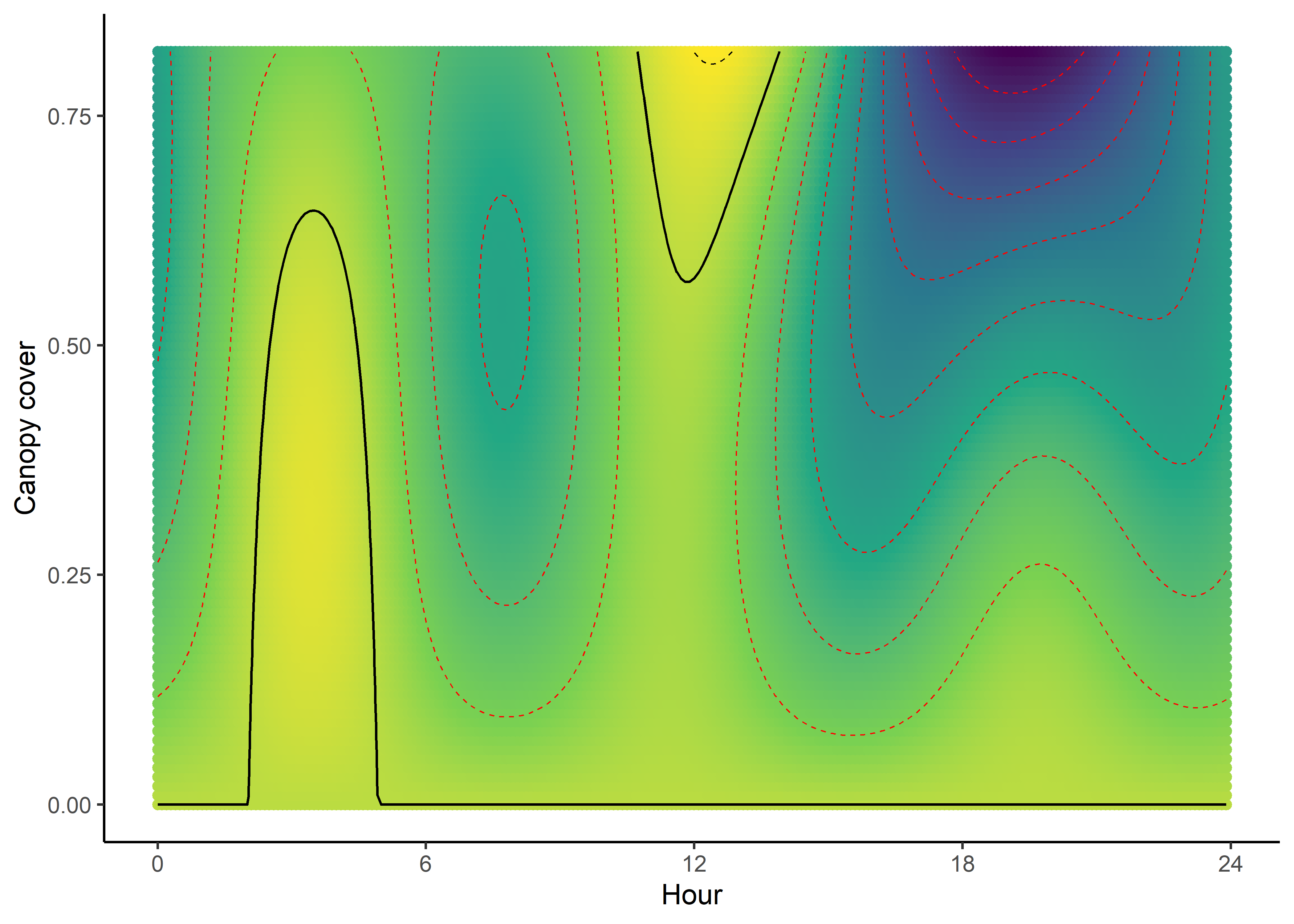
Code
canopy_min <- min(buffalo_data$canopy_01, na.rm = TRUE)
canopy_max <- max(buffalo_data$canopy_01, na.rm = TRUE)
canopy_seq <- seq(canopy_min, canopy_max, by = 0.01)

# Create empty data frame
canopy_fresponse_df <- data.frame(matrix(ncol = nrow(hour_coefs_nat_df_3p),
                                         nrow = length(canopy_seq)))

for(i in 1:nrow(hour_coefs_nat_df_3p)) {
  # Assign the vector as a column to the dataframe
  canopy_fresponse_df[,i] <- (hour_coefs_nat_df_3p$canopy[i] * canopy_seq) +
    (hour_coefs_nat_df_3p$canopy_2[i] * (canopy_seq ^ 2))
}

canopy_fresponse_df <- data.frame(canopy_seq, canopy_fresponse_df)
colnames(canopy_fresponse_df) <- c("canopy", hour)
canopy_fresponse_long <- pivot_longer(canopy_fresponse_df, cols = !1,
                                      names_to = "hour")

canopy_contour_min <- min(canopy_fresponse_long$value) # 0
canopy_contour_max <- max(canopy_fresponse_long$value) # 2.181749
canopy_contour_increment <- (canopy_contour_max-canopy_contour_min)/10

canopy_quad_3p <- ggplot(data = canopy_fresponse_long,
                         aes(x = as.numeric(hour), y = canopy)) +
  geom_point(aes(colour = value)) +
  geom_contour(aes(z = value),
               breaks = seq(canopy_contour_increment,
                            canopy_contour_max,
                            canopy_contour_increment),
               colour = "black", linewidth = 0.25, linetype = "dashed") +
  geom_contour(aes(z = value),
               breaks = seq(-canopy_contour_increment,
                            canopy_contour_min,
                            -canopy_contour_increment),
               colour = "red", linewidth = 0.25, linetype = "dashed") +
  geom_contour(aes(z = value), breaks = 0, colour = "black", linewidth = 0.5) +
  scale_x_continuous("Hour", breaks = seq(0,24,6)) +
  scale_y_continuous("Canopy cover", breaks = seq(0, 1, 0.25)) +
  scale_colour_viridis_c("Selection") +
  # ggtitle("Canopy Cover",
  #         subtitle = "Three pairs of harmonics") +
  theme_classic() +
  theme(legend.position = "none")

canopy_quad_3p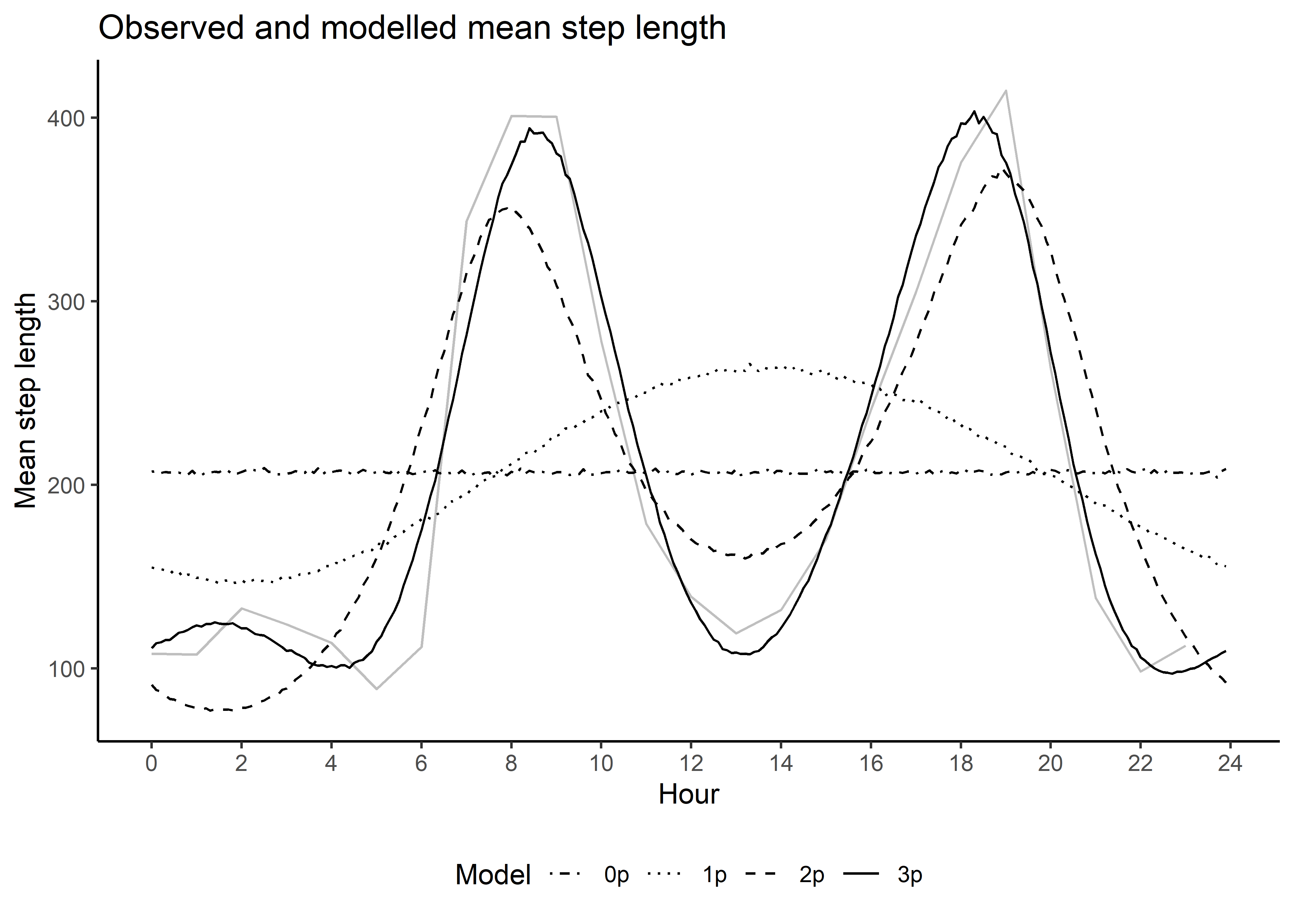
Combining the plots
Movement parameters
Code
gamma_df <- rbind(gamma_df_0p, gamma_df_1p, gamma_df_2p, gamma_df_3p)
gamma_df <- gamma_df %>% mutate(model_f = as.numeric(factor(model)))

mean_sl <- ggplot() +
  geom_path(data = movement_summary_buffalo,
            aes(x = hour, y = mean_sl, group = factor(id)),
            alpha = 0.25) +
  geom_path(data = gamma_df, aes(x = hour, y = mean, linetype = model)) +
  scale_x_continuous("Hour", breaks = seq(0,24,2)) +
  scale_y_continuous("Mean step length") +
  scale_linetype_manual("Model", breaks=c("0p","1p", "2p", "3p"),
                        values=c(4,3,2,1)) +
  ggtitle("Observed and modelled mean step length") +
  theme_classic() +
  theme(legend.position = "bottom")

mean_sl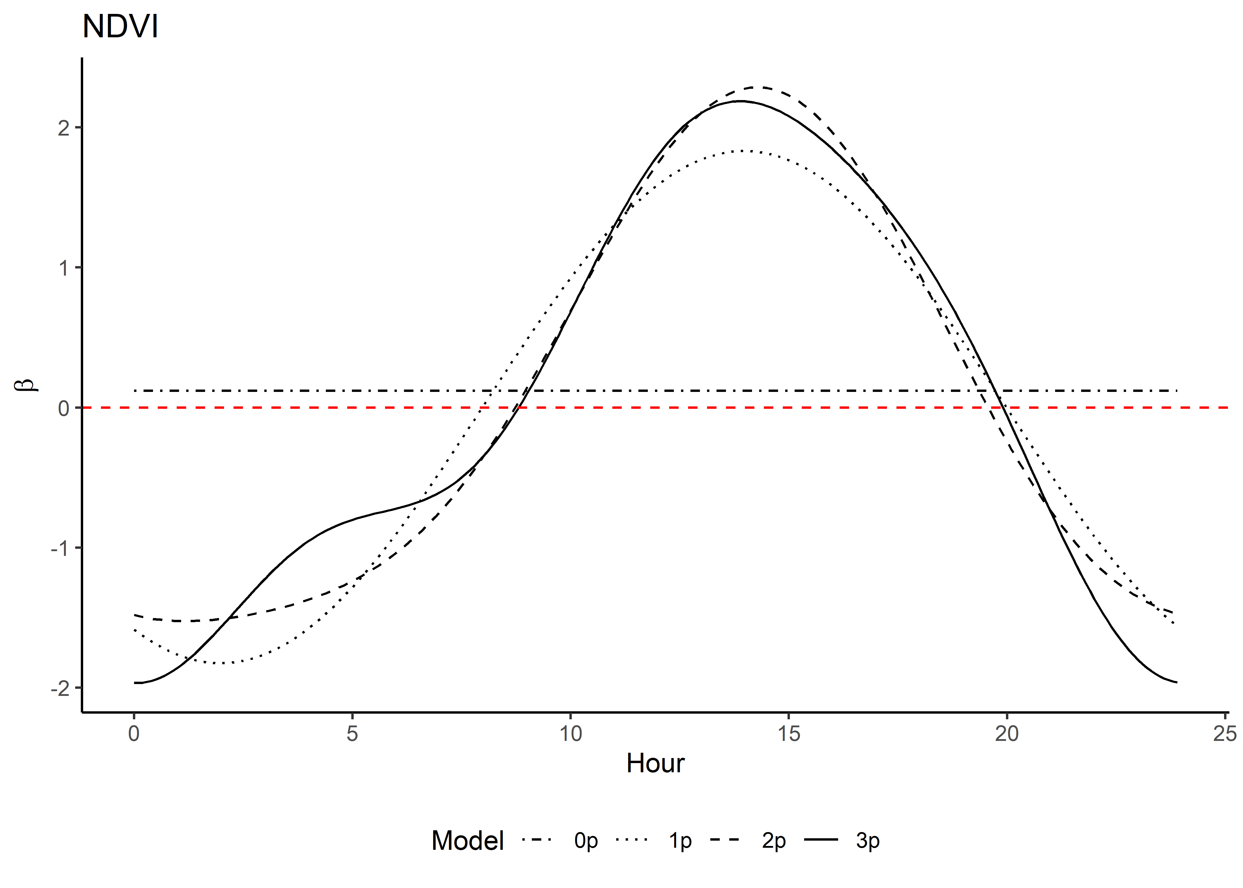
Code
# ggsave(paste0("outputs/plots/manuscript_figs_R1/mean_sl_",
#          Sys.Date(), ".png"),
#   width=150, height=90, units="mm", dpi = 1000)

median_sl <- ggplot() +
  geom_path(data = movement_summary_buffalo,
            aes(x = hour, y = median_sl, group = factor(id)),
            alpha = 0.25) +
  geom_path(data = gamma_df, aes(x = hour, y = median, linetype = model)) +
  scale_x_continuous("Hour", breaks = seq(0,24,2)) +
  scale_y_continuous("Median step length") +
  scale_linetype_manual("Model", breaks=c("0p","1p", "2p", "3p"),
                        values=c(4,3,2,1)) +
  ggtitle("Observed and modelled median step length") +
  theme_classic() +
  theme(legend.position = "bottom")

median_sl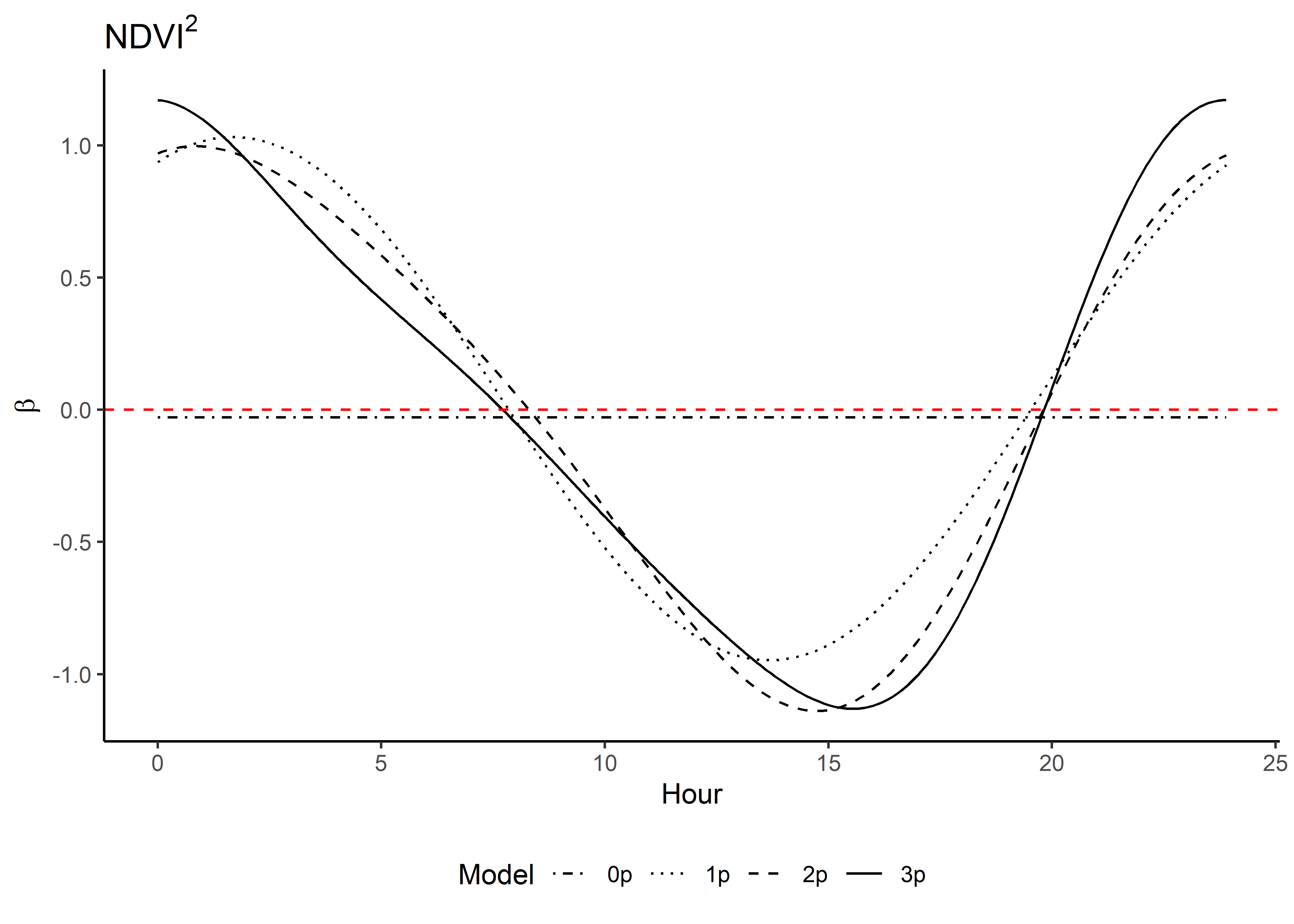
Habitat selection
Code
harmonics_scaled_long_0p <- harmonics_scaled_long_0p %>% mutate(model = "0p")
harmonics_scaled_long_1p <- harmonics_scaled_long_1p %>% mutate(model = "1p")
harmonics_scaled_long_2p <- harmonics_scaled_long_2p %>% mutate(model = "2p")
harmonics_scaled_long_3p <- harmonics_scaled_long_3p %>% mutate(model = "3p")

harmonics_scaled_long_Mp <- rbind(harmonics_scaled_long_0p,
                                  harmonics_scaled_long_1p,
                                  harmonics_scaled_long_2p,
                                  harmonics_scaled_long_3p)

coef_titles <- unique(harmonics_scaled_long_Mp$coef)


ndvi_harms <- ggplot() +
      geom_path(data = harmonics_scaled_long_Mp %>%
                filter(coef == "ndvi"),
                aes(x = hour, y = value, linetype = model)) +
      geom_hline(yintercept = 0, linetype = "dashed", colour = "red") +
      scale_y_continuous(expression(beta)) +
      scale_x_continuous("Hour") +
  scale_linetype_manual("Model", breaks=c("0p","1p", "2p", "3p"),
                        values=c(4,3,2,1)) +
      ggtitle("NDVI") +
      theme_classic() +
      theme(legend.position = "bottom")

ndvi_harms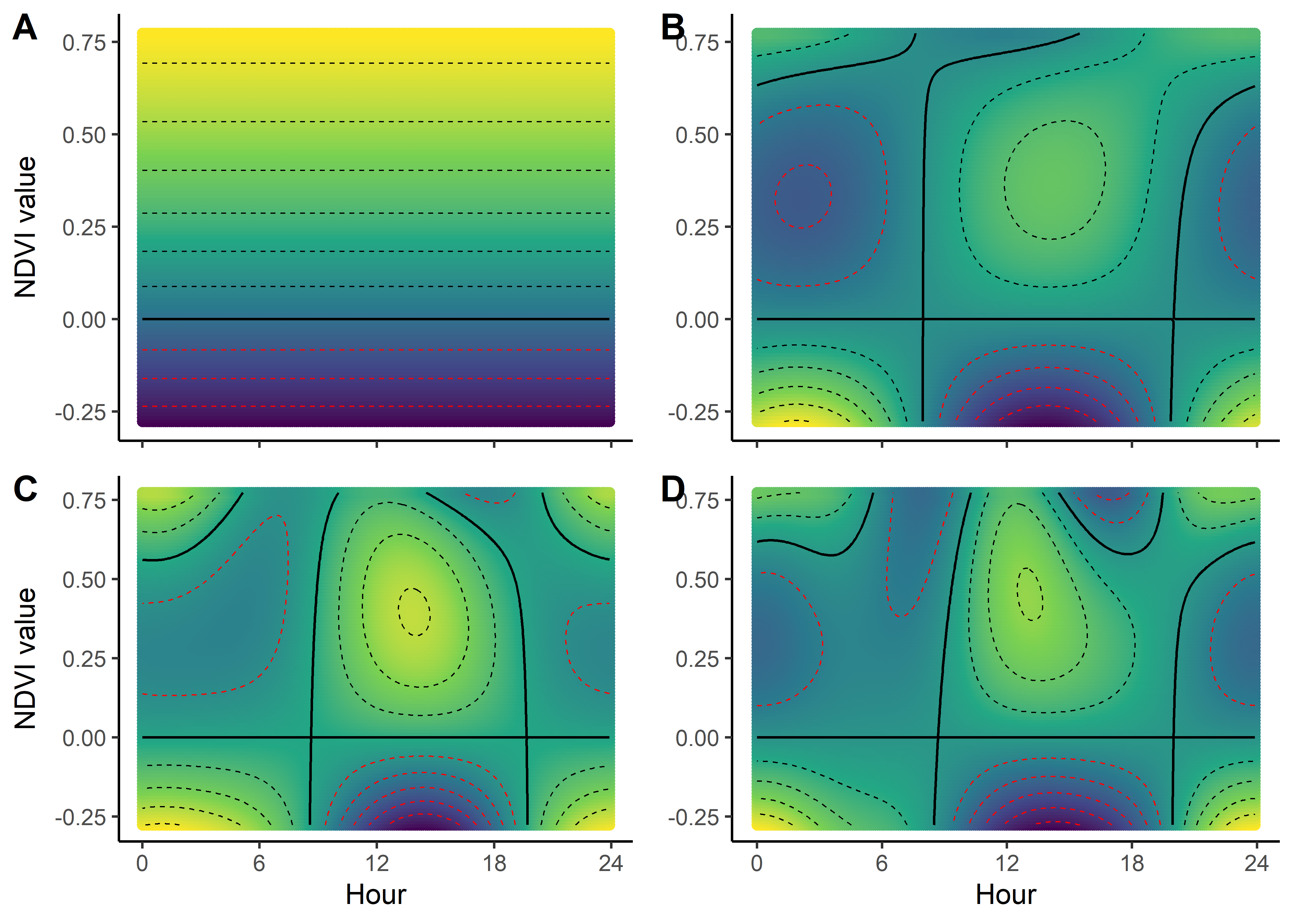
Code
ndvi_2_harms <- ggplot() +
      geom_path(data = harmonics_scaled_long_Mp %>%
                filter(coef == "ndvi_2"),
                aes(x = hour, y = value, linetype = model)) +
      geom_hline(yintercept = 0, linetype = "dashed", colour = "red") +
      scale_y_continuous(expression(beta)) +
      scale_x_continuous("Hour") +
  scale_linetype_manual("Model", breaks=c("0p","1p", "2p", "3p"),
                        values=c(4,3,2,1)) +
      ggtitle(expression(NDVI^2)) +
      theme_classic() +
      theme(legend.position = "bottom")

ndvi_2_harms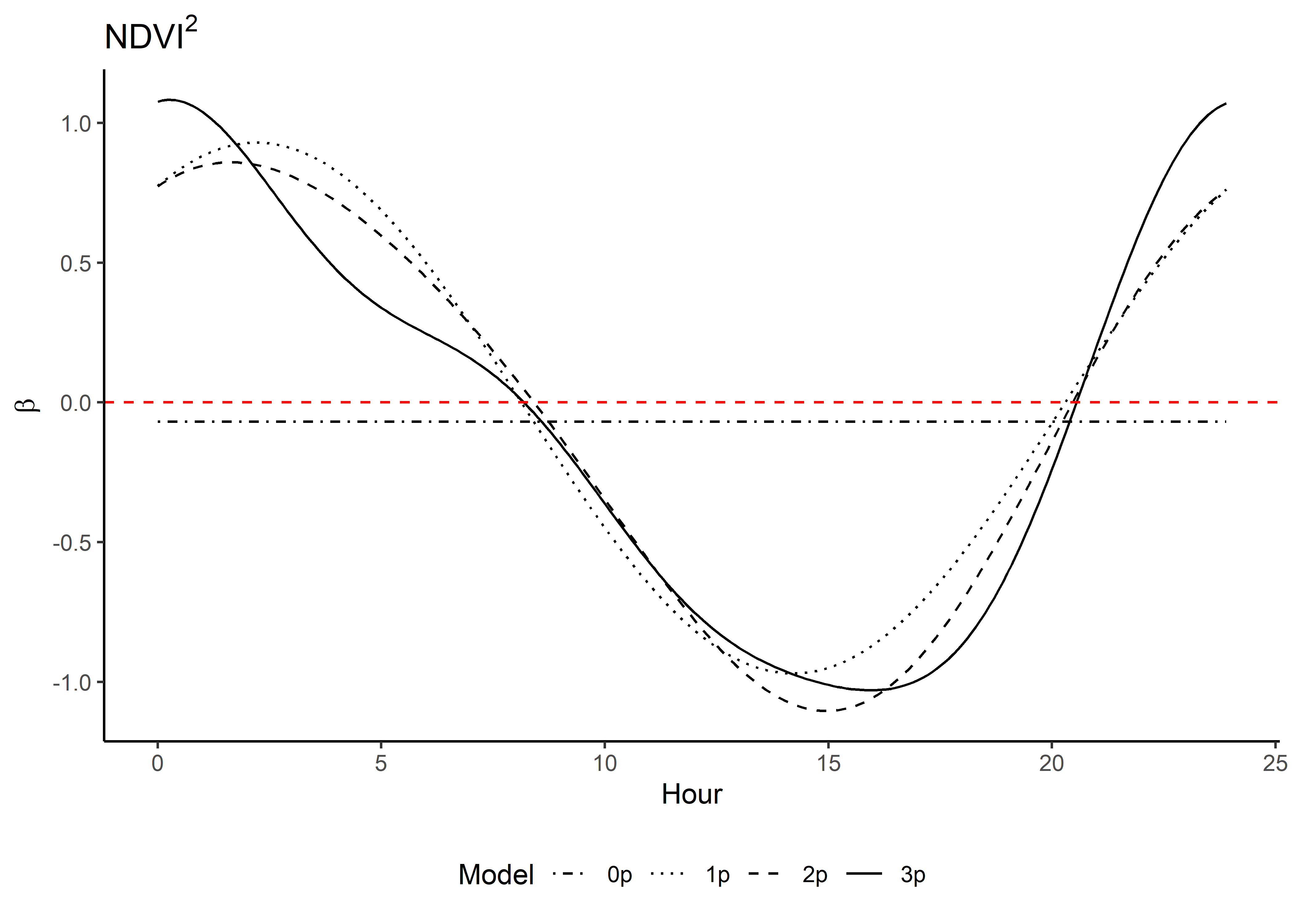
Code
canopy_harms <- ggplot() +
      geom_path(data = harmonics_scaled_long_Mp %>%
                filter(coef == "canopy"),
                aes(x = hour, y = value, linetype = model)) +
      geom_hline(yintercept = 0, linetype = "dashed", colour = "red") +
      scale_y_continuous(expression(beta)) +
      scale_x_continuous("Hour") +
  scale_linetype_manual("Model", breaks=c("0p","1p", "2p", "3p"),
                        values=c(4,3,2,1)) +
      ggtitle("Canopy cover") +
      theme_classic() +
      theme(legend.position = "bottom")

canopy_harms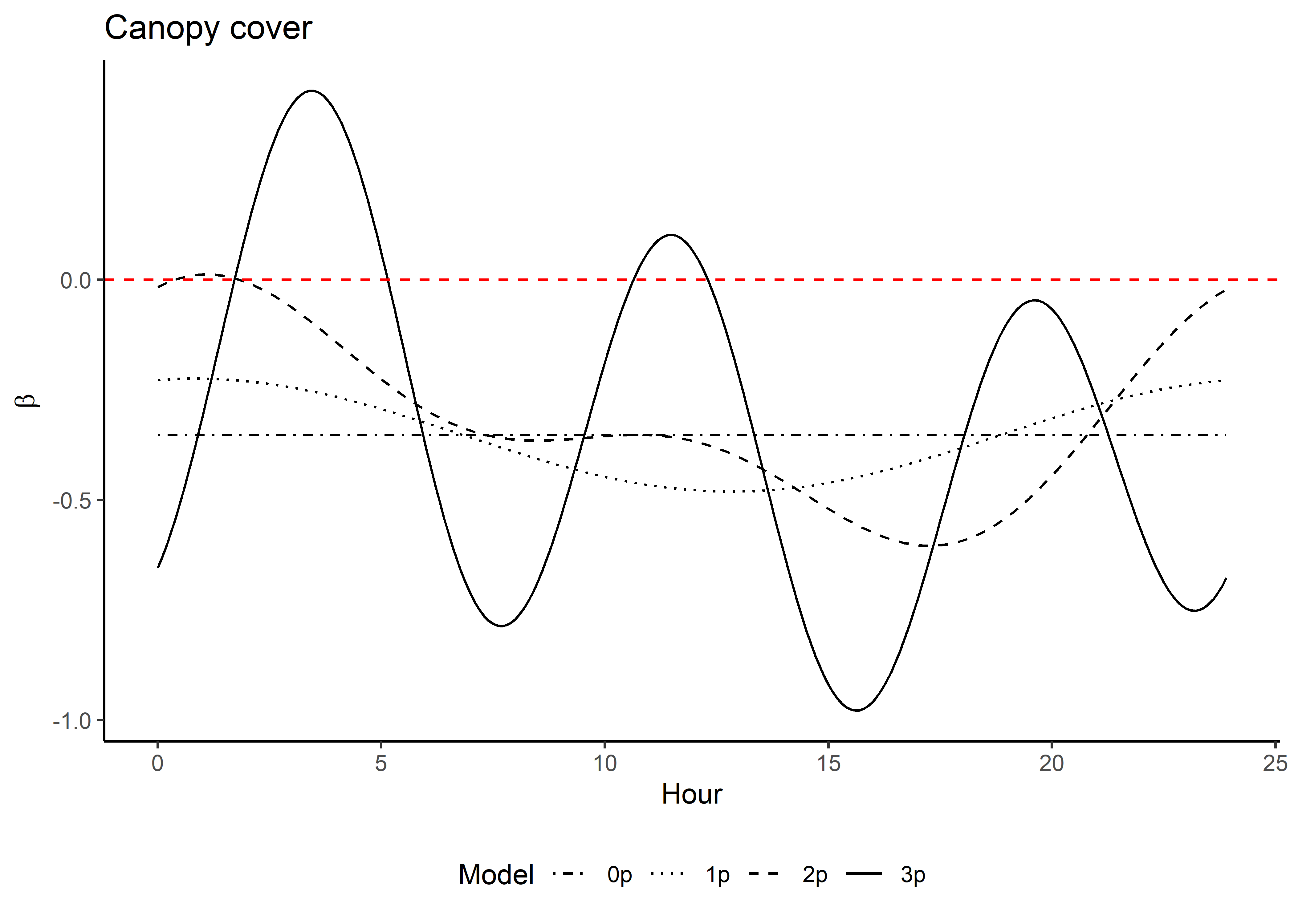
Code
canopy_2_harms <- ggplot() +
      geom_path(data = harmonics_scaled_long_Mp %>%
                filter(coef == "canopy_2"),
                aes(x = hour, y = value, linetype = model)) +
      geom_hline(yintercept = 0, linetype = "dashed", colour = "red") +
      scale_y_continuous(expression(beta)) +
      scale_x_continuous("Hour") +
  scale_linetype_manual("Model", breaks=c("0p","1p", "2p", "3p"),
                        values=c(4,3,2,1)) +
      ggtitle(expression(Canopy~cover^2)) +
      theme_classic() +
      theme(legend.position = "bottom")

canopy_2_harms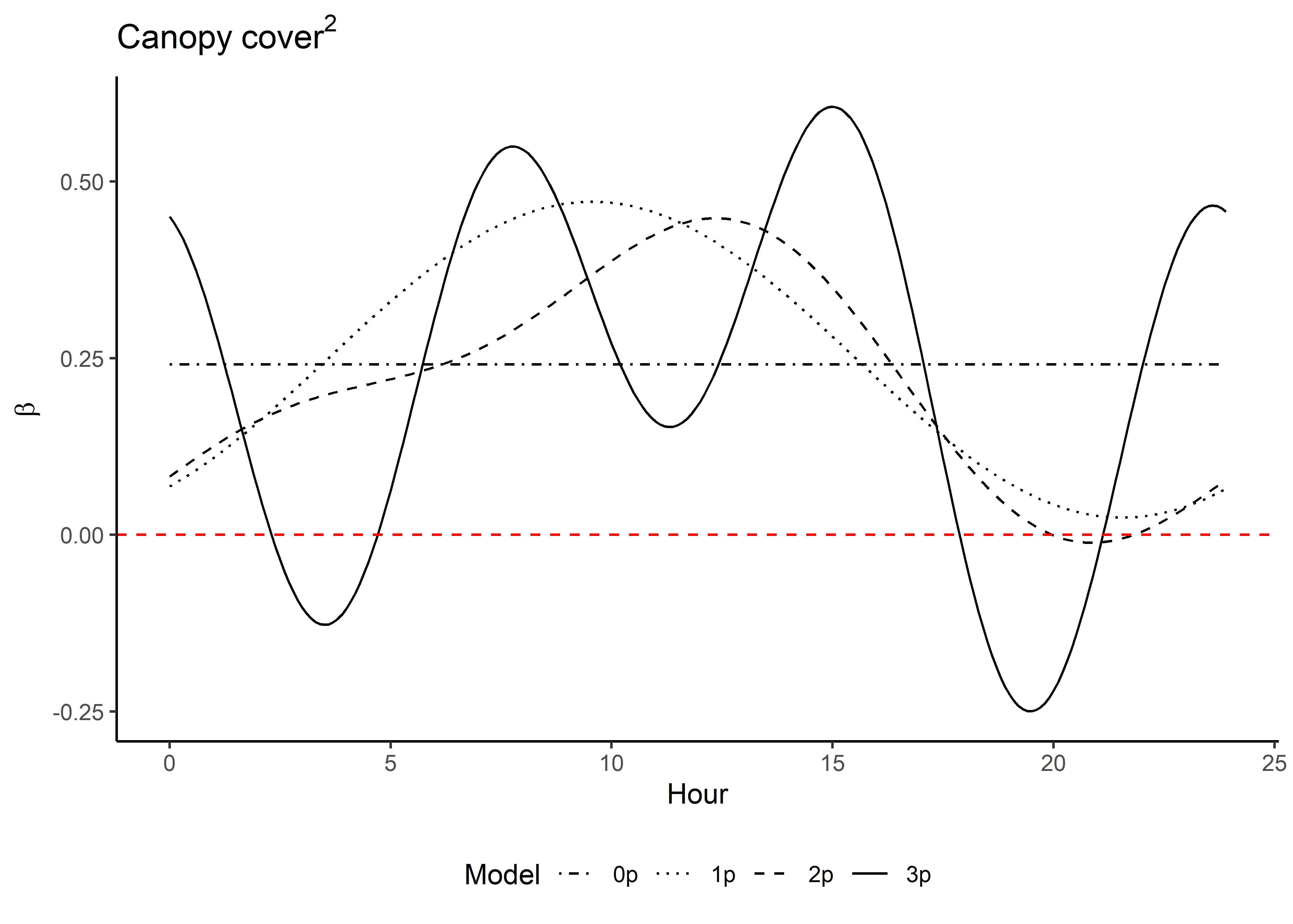
Code
herby_harms <- ggplot() +
      geom_path(data = harmonics_scaled_long_Mp %>%
                filter(coef == "herby"),
                aes(x = hour, y = value, linetype = model)) +
      geom_hline(yintercept = 0, linetype = "dashed", colour = "red") +
      scale_y_continuous(expression(beta), limits = c(-0.4,0.15)) +
      scale_x_continuous("Hour") +
  scale_linetype_manual("Model", breaks=c("0p","1p", "2p", "3p"),
                        values=c(4,3,2,1)) +
      ggtitle("Herbaceous vegetation") +
      theme_classic() +
      theme(legend.position = "bottom")

herby_harms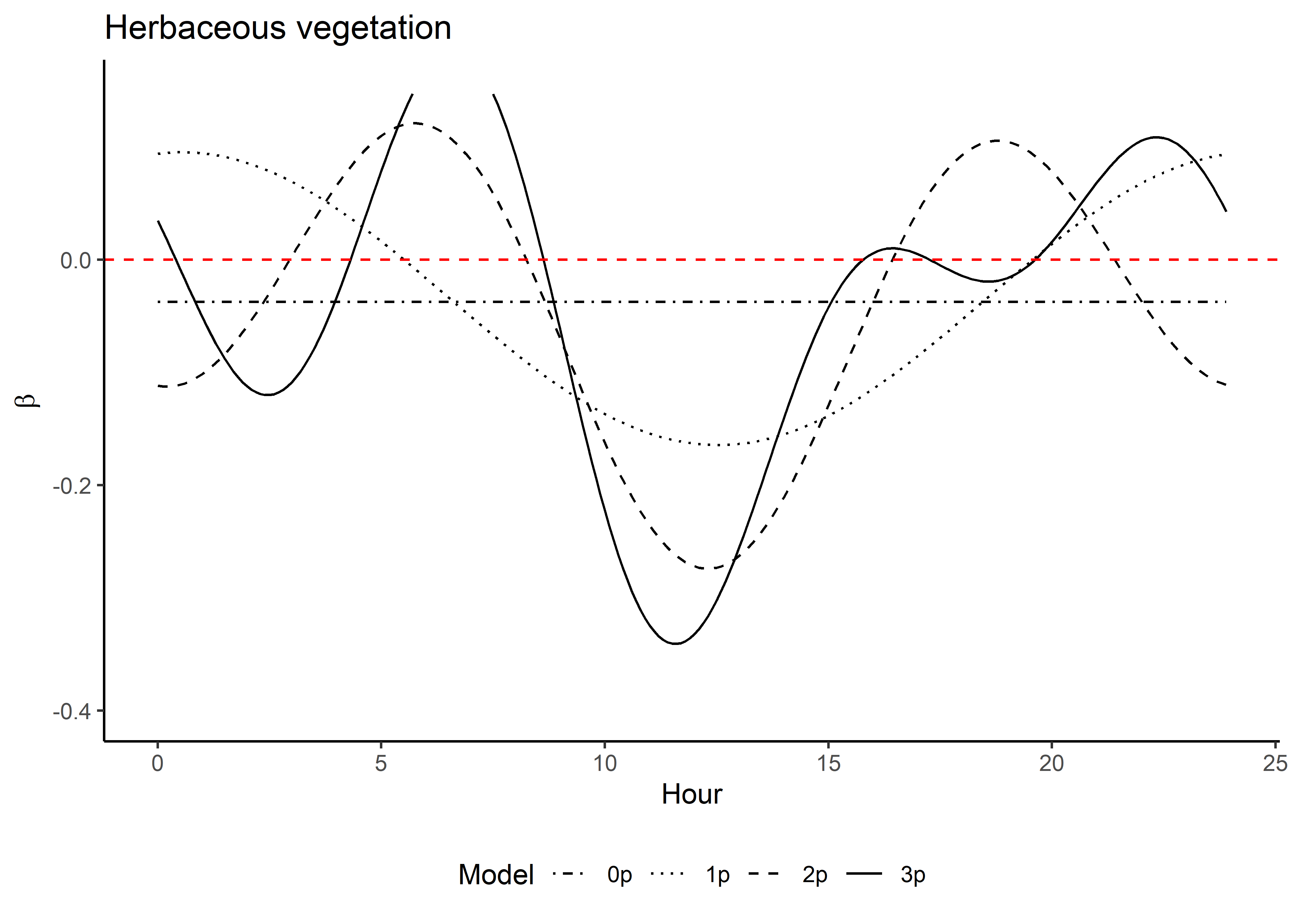
Code
slope_harms <- ggplot() +
      geom_path(data = harmonics_scaled_long_Mp %>%
                filter(coef == "slope"),
                aes(x = hour, y = value, linetype = model)) +
      geom_hline(yintercept = 0, linetype = "dashed", colour = "red") +
      scale_y_continuous(expression(beta), limits = c(-0.4,0.15)) +
      scale_x_continuous("Hour") +
  scale_linetype_manual("Model", breaks=c("0p","1p", "2p", "3p"),
                        values=c(4,3,2,1)) +
      ggtitle("Slope") +
      theme_classic() +
      theme(legend.position = "bottom")

slope_harms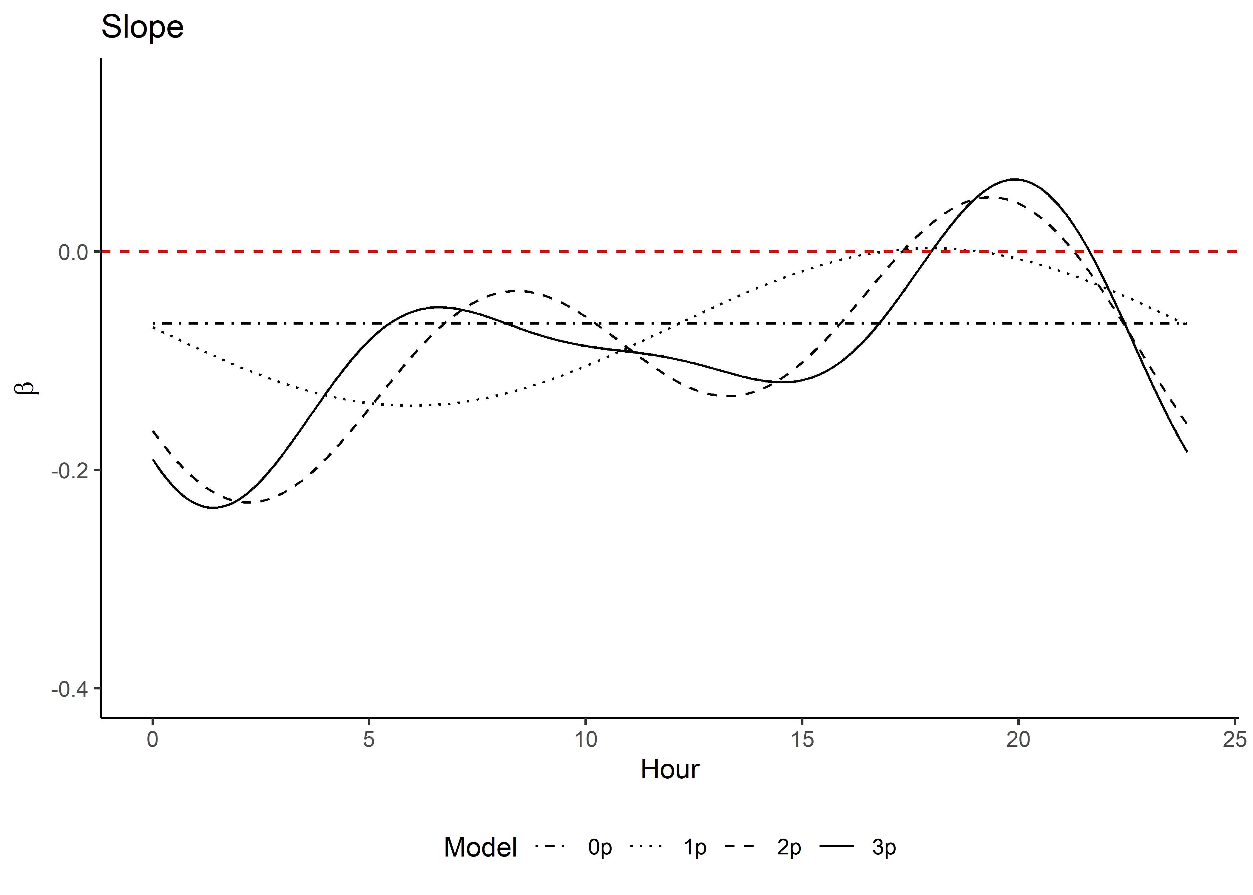
Code
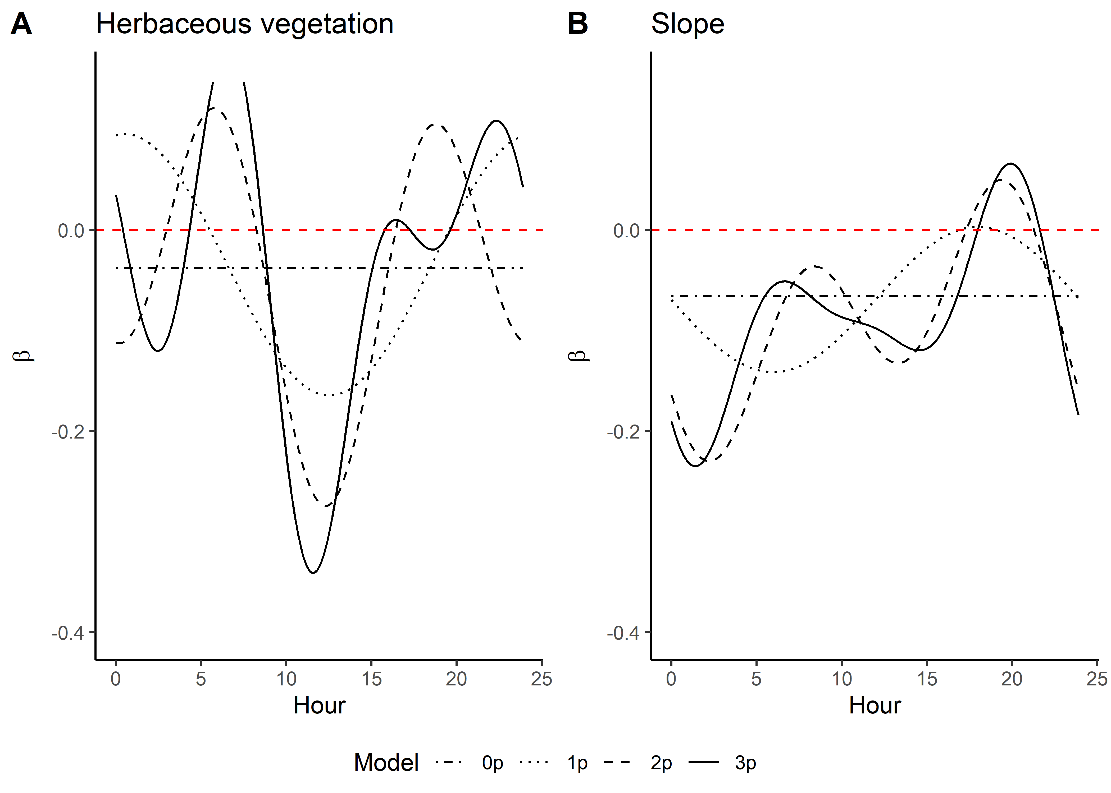
Combining selection surfaces
NDVI
- A = 0p model
- B = 1p model
- C = 2p model
- D = 3p model
Code
ggarrange(ndvi_quad_0p + theme(plot.title = element_blank(),
                               axis.title.x = element_blank(),
                               axis.text.x = element_blank()),

          ndvi_quad_1p + theme(plot.title = element_blank(),
                               axis.title.x = element_blank(),
                               axis.text.x = element_blank(),
                               axis.title.y = element_blank(),
                               ),

          ndvi_quad_2p,

          ndvi_quad_3p + theme(plot.title = element_blank(),
                               axis.title.y = element_blank(),
                               ),

          labels = c("A", "B", "C", "D"),
          ncol = 2, nrow = 2,
          legend = "none",
          common.legend = TRUE)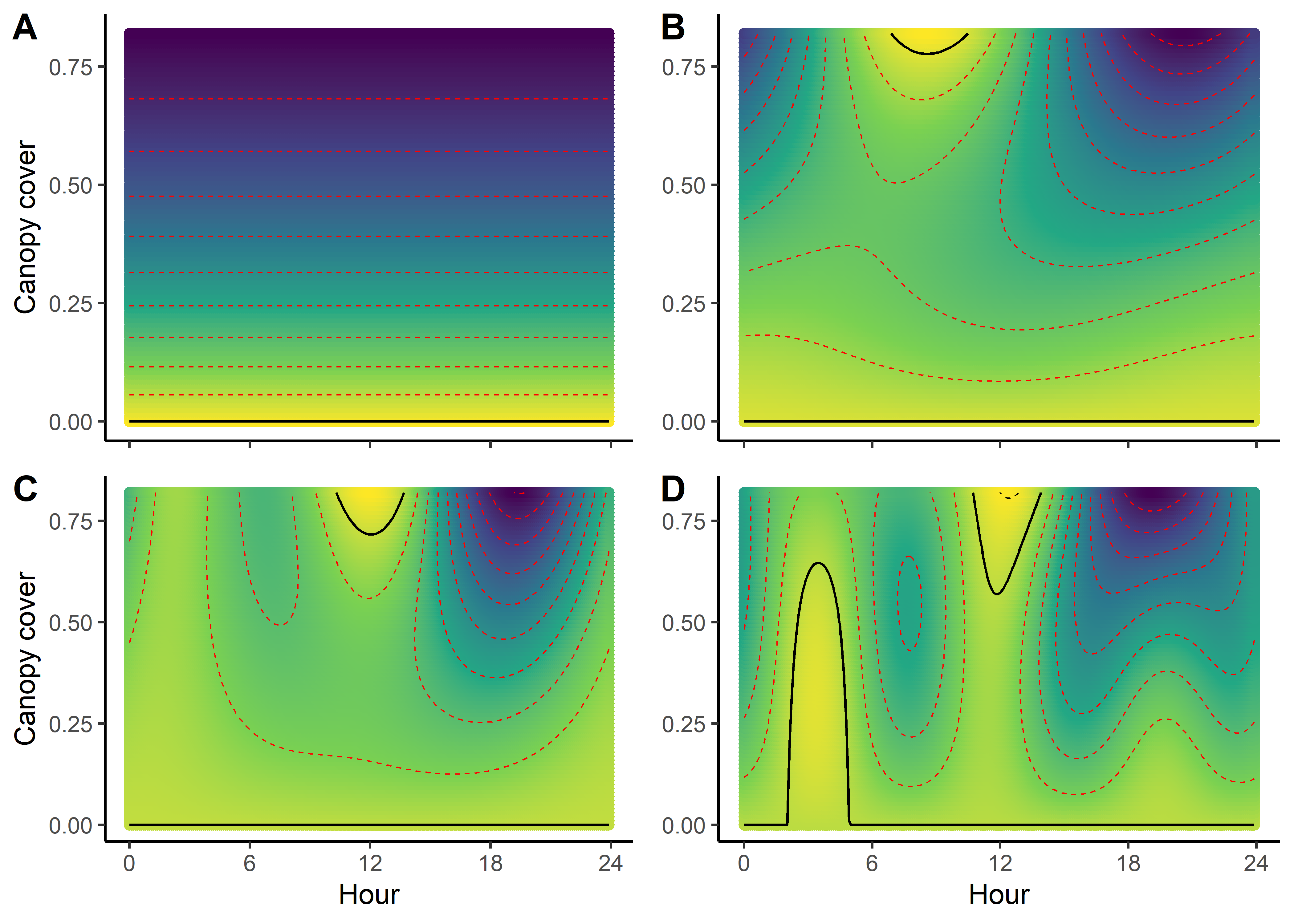
Canopy cover
- A = 0p model
- B = 1p model
- C = 2p model
- D = 3p model
Code
ggarrange(canopy_quad_0p + theme(plot.title = element_blank(),
                               axis.title.x = element_blank(),
                               axis.text.x = element_blank()),

          canopy_quad_1p + theme(plot.title = element_blank(),
                               axis.title.x = element_blank(),
                               axis.text.x = element_blank(),
                               axis.title.y = element_blank(),
                               ),

          canopy_quad_2p,

          canopy_quad_3p + theme(plot.title = element_blank(),
                               axis.title.y = element_blank(),
                               ),

          labels = c("A", "B", "C", "D"),
          ncol = 2, nrow = 2,
          legend = "none",
          common.legend = TRUE)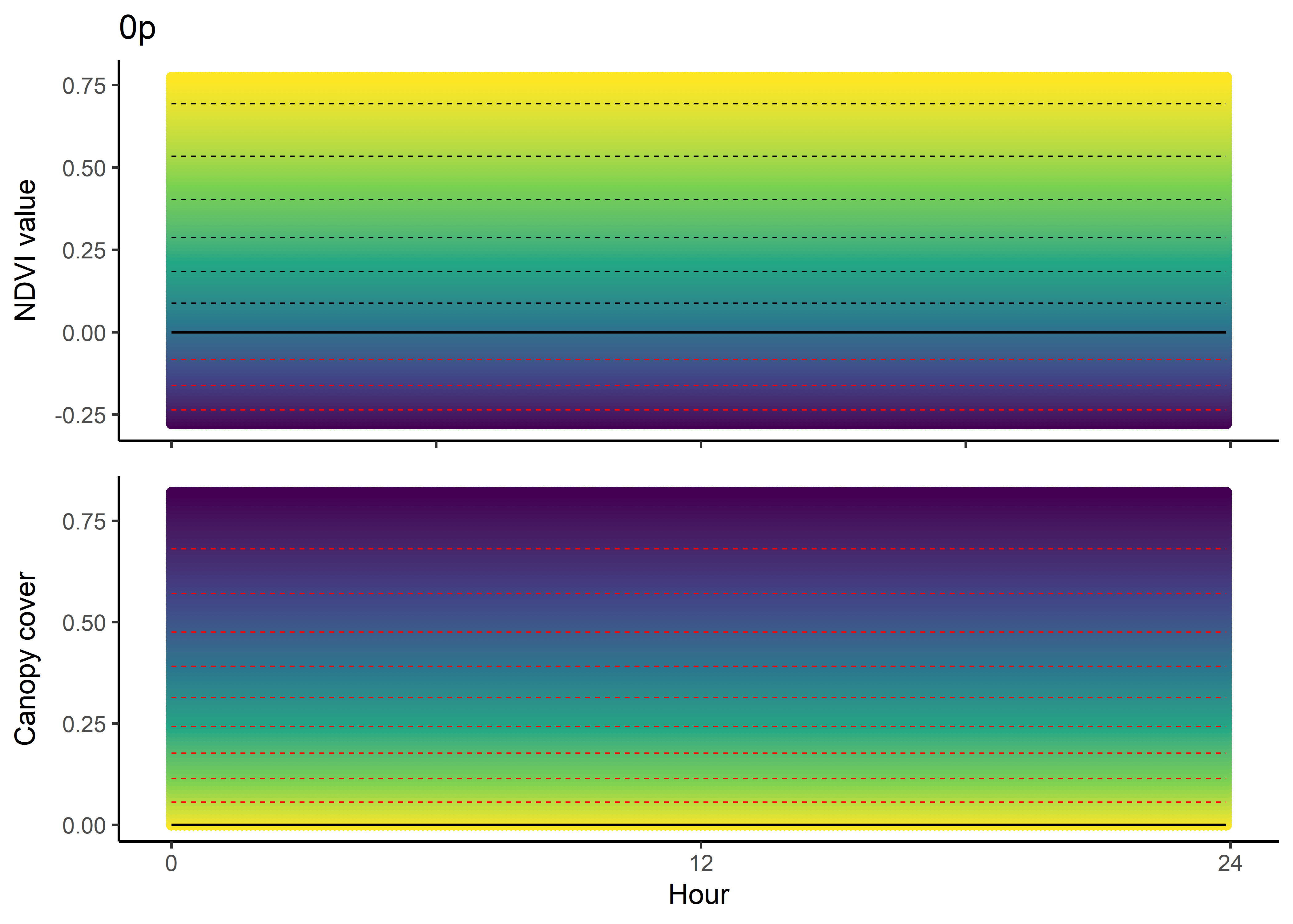
Adding all selection surfaces to the same plot
We combine these plots into the plot that is in the paper. On the top is the NDVI selection surface, and on the bottom is the canopy cover selection surface.
Code
surface_plots_0p <- ggarrange(ndvi_quad_0p +
            ggtitle("0p") +
            theme(axis.title.x = element_blank(),
                  axis.text.x = element_blank()),

          canopy_quad_0p +
            scale_x_continuous("Hour", breaks = c(0,12,24)) +
            theme(plot.title = element_blank()),

          ncol = 1, nrow = 2,
          align = "v",
          legend = "none",
          common.legend = TRUE)
Scale for x is already present.
Adding another scale for x, which will replace the existing scale.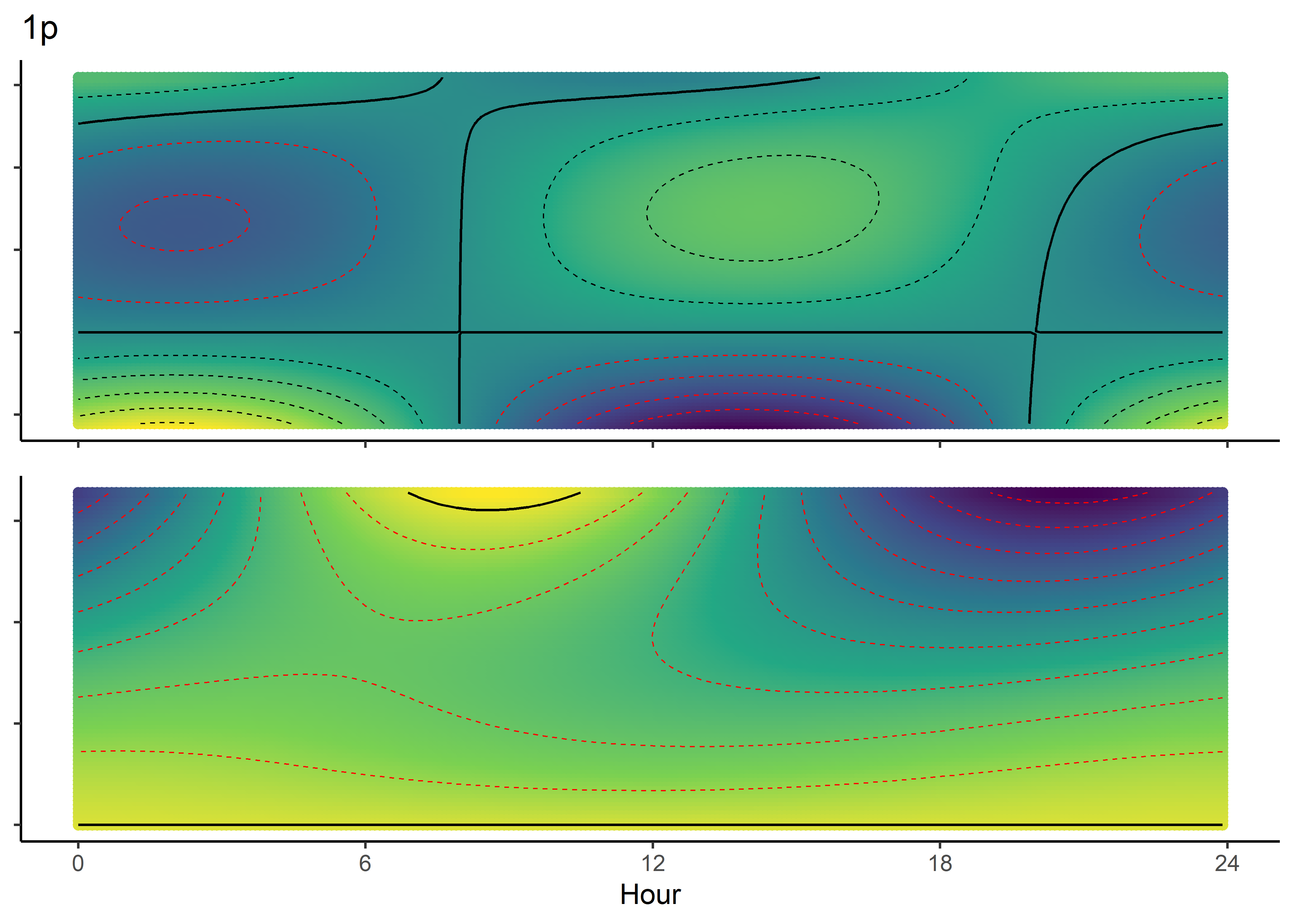
Code
surface_plots_1p <- ggarrange(ndvi_quad_1p +
            ggtitle("1p") +
            theme(axis.title.x = element_blank(),
                  axis.text.x = element_blank(),
                  axis.title.y = element_blank(),
                  axis.text.y = element_blank()),

          canopy_quad_1p +
            theme(plot.title = element_blank(),
                  axis.title.y = element_blank(),
                  axis.text.y = element_blank()),

          ncol = 1, nrow = 2,
          align = "v",
          legend = "none",
          common.legend = TRUE)

surface_plots_1p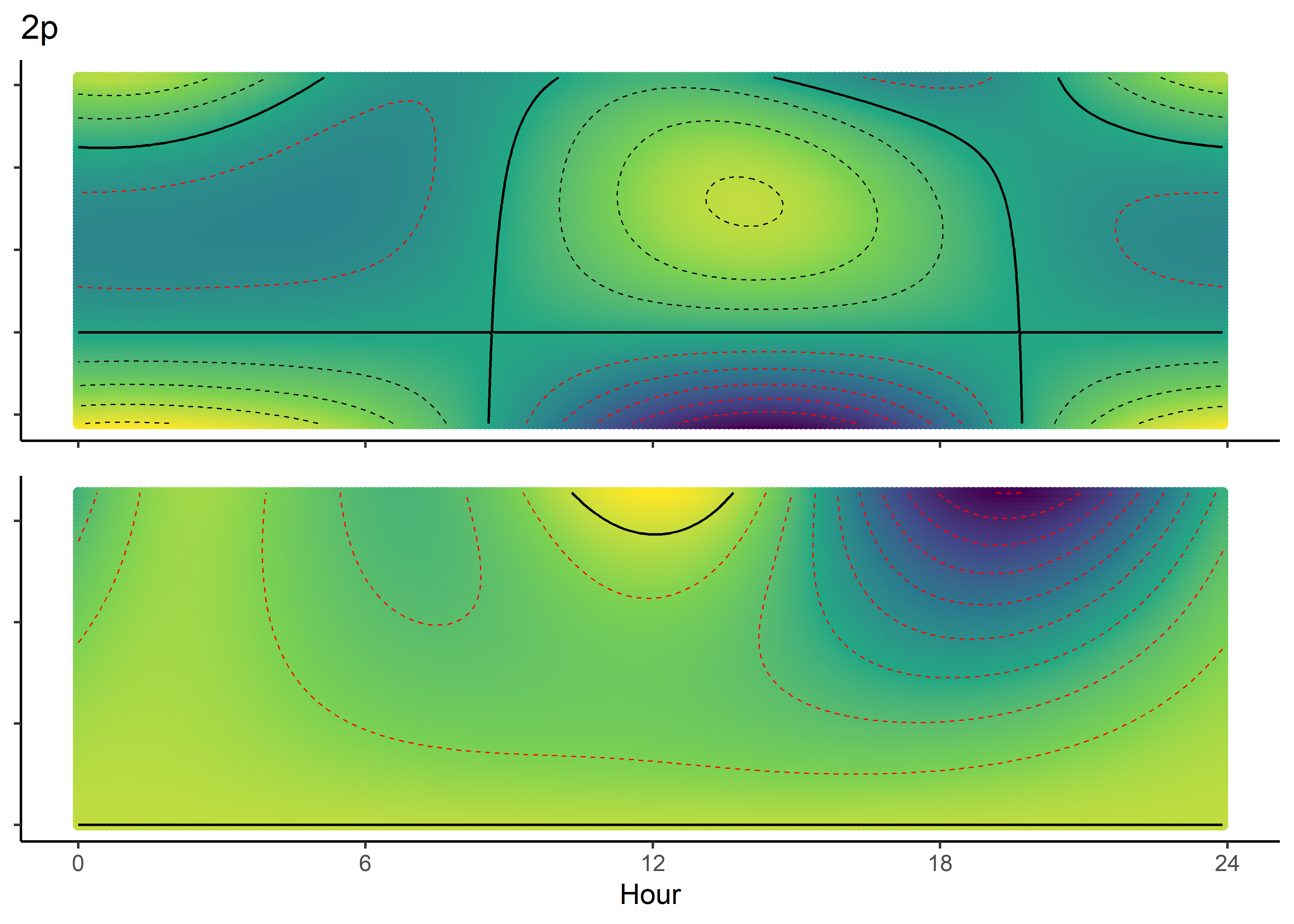
Code
surface_plots_2p <- ggarrange(ndvi_quad_2p +
            ggtitle("2p") +
            theme(axis.title.x = element_blank(),
                  axis.text.x = element_blank(),
                  axis.title.y = element_blank(),
                  axis.text.y = element_blank()),

          canopy_quad_2p +
            theme(plot.title = element_blank(),
                  axis.title.y = element_blank(),
                  axis.text.y = element_blank()),

          ncol = 1, nrow = 2,
          align = "v",
          legend = "none",
          common.legend = TRUE)

surface_plots_2p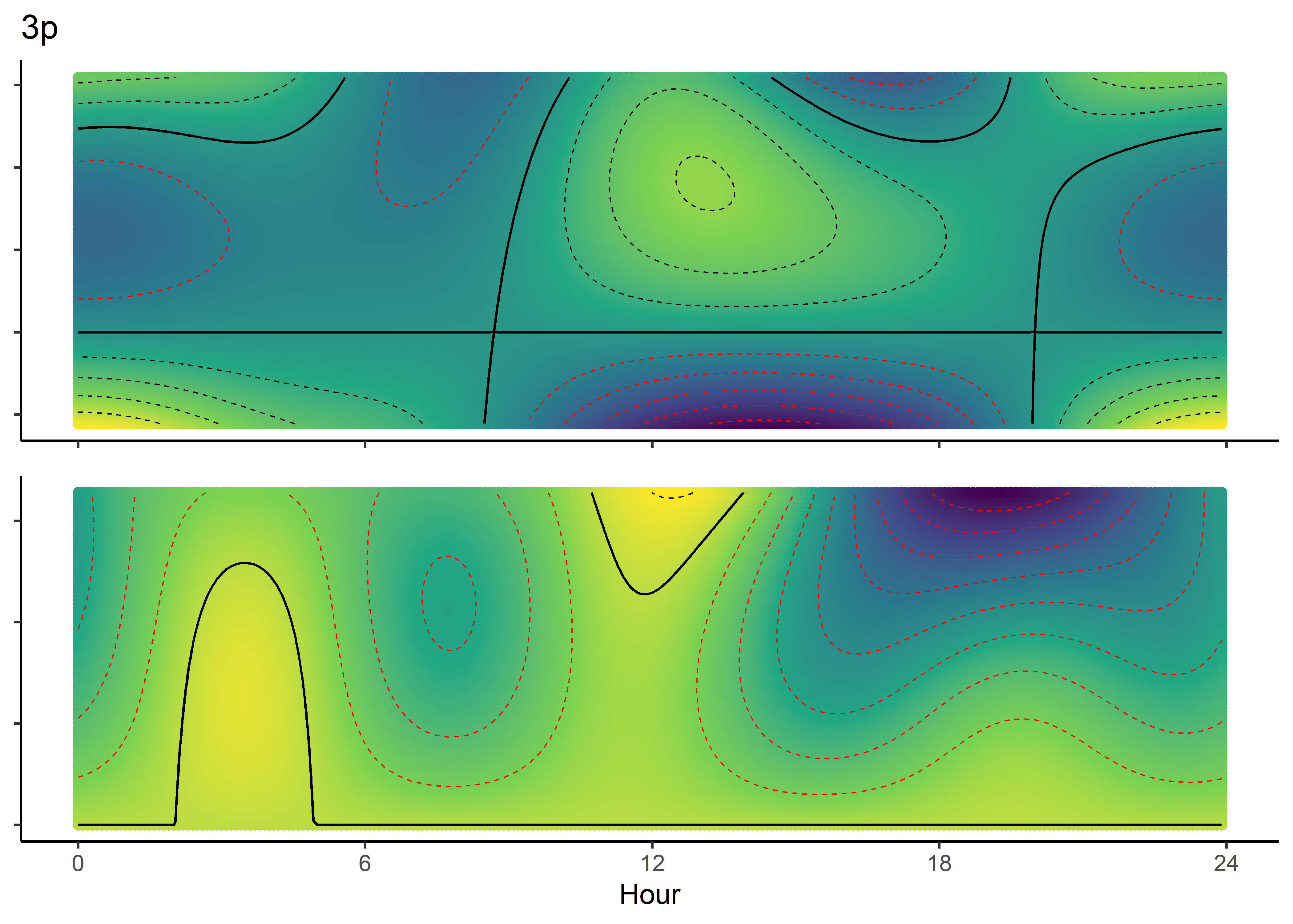
Code
surface_plots_3p <- ggarrange(ndvi_quad_3p +
            ggtitle("3p") +
              theme(axis.title.x = element_blank(),
                    axis.text.x = element_blank(),
                    axis.title.y = element_blank(),
                    axis.text.y = element_blank()),

           canopy_quad_3p +
            theme(plot.title = element_blank(),
                  axis.title.y = element_blank(),
                  axis.text.y = element_blank()),

          ncol = 1, nrow = 2,
          align = "v",
          legend = "none",
          common.legend = TRUE)

surface_plots_3p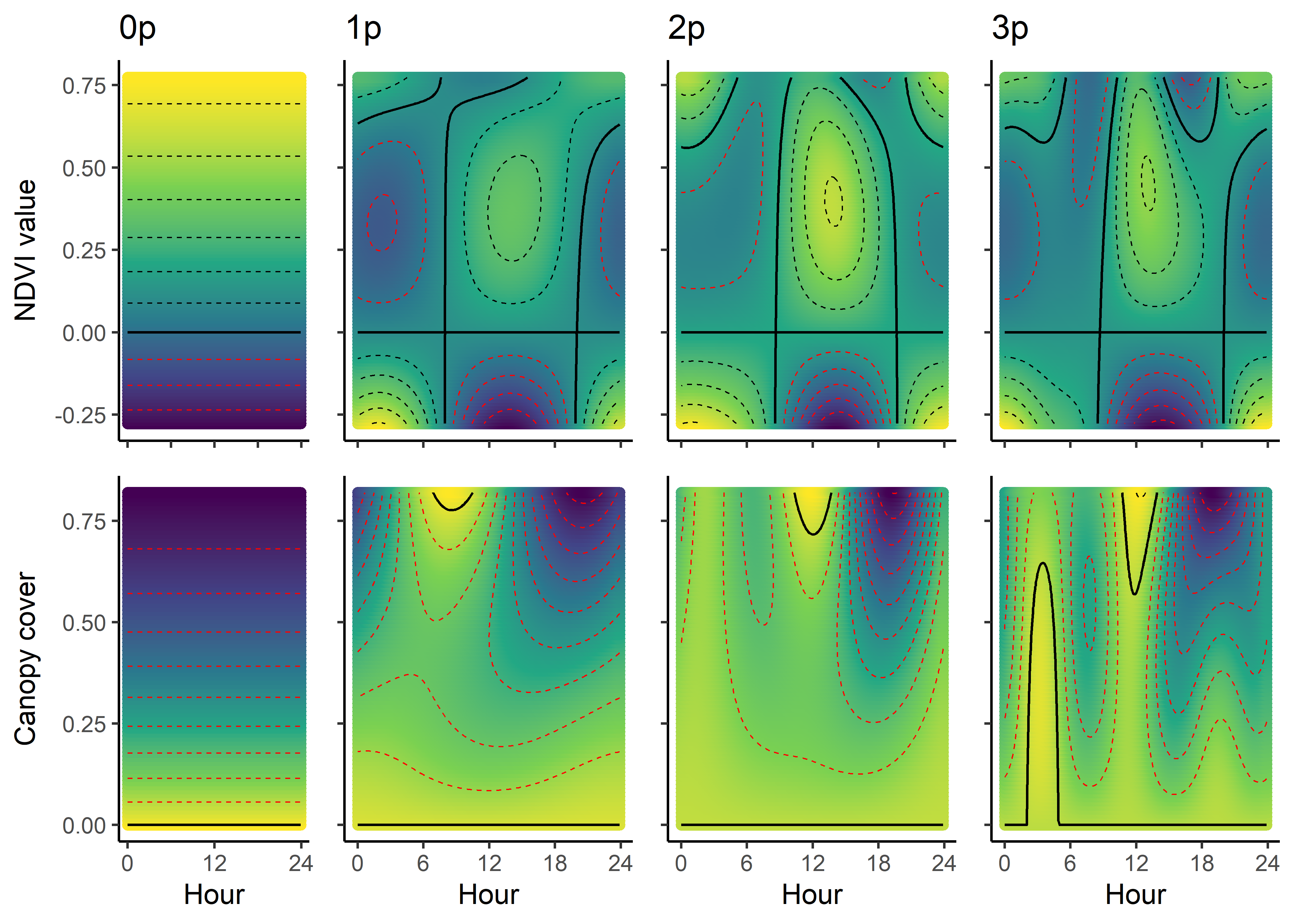
All selection surfaces
Code
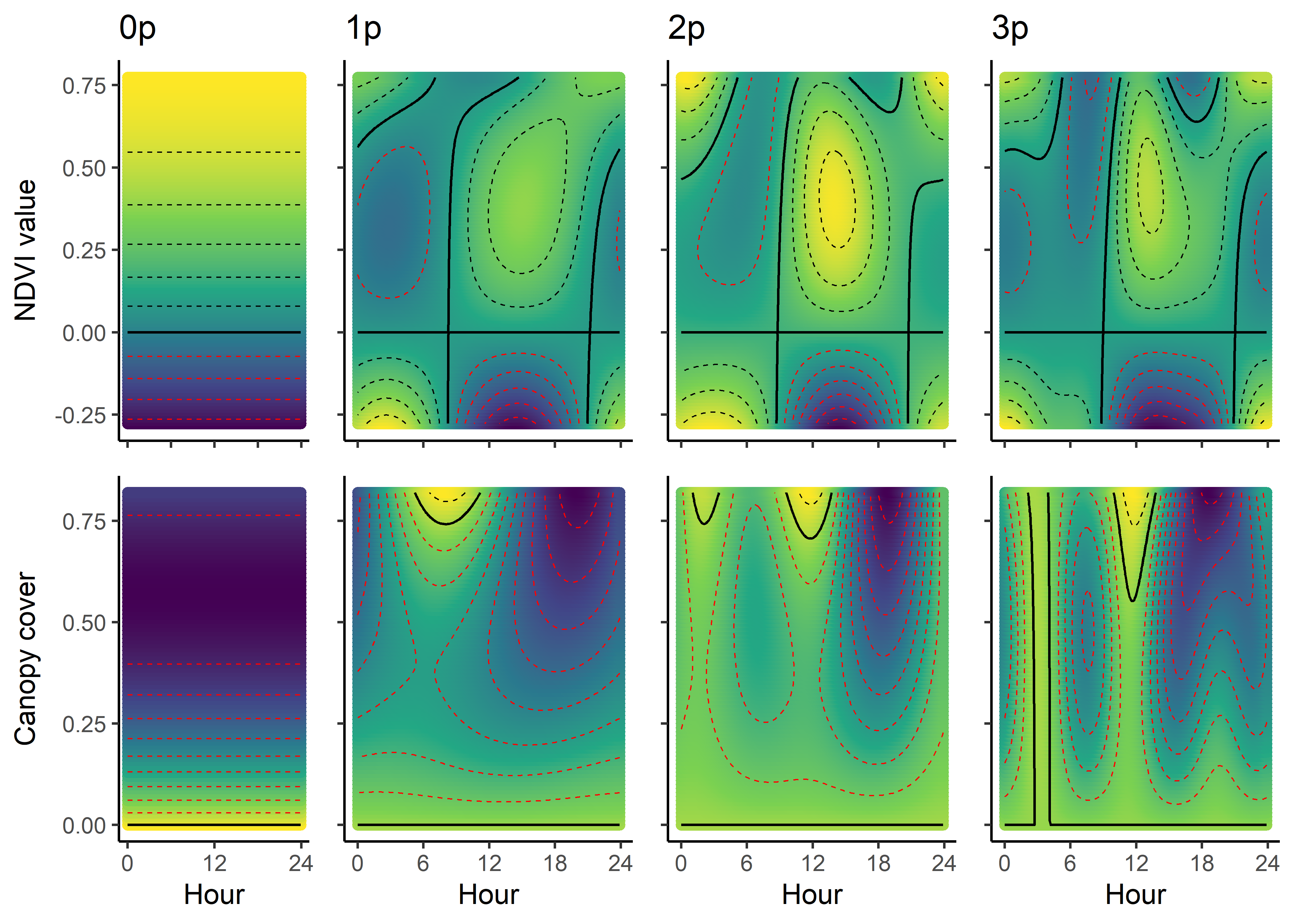
References
Session info
R version 4.4.1 (2024-06-14 ucrt)
Platform: x86_64-w64-mingw32/x64
Running under: Windows 11 x64 (build 22631)

Matrix products: default


locale:
[1] LC_COLLATE=English_Australia.utf8  LC_CTYPE=English_Australia.utf8
[3] LC_MONETARY=English_Australia.utf8 LC_NUMERIC=C
[5] LC_TIME=English_Australia.utf8

time zone: America/Los_Angeles
tzcode source: internal

attached base packages:
[1] stats     graphics  grDevices utils     datasets  methods   base

other attached packages:
 [1] ggpubr_0.6.0    beepr_2.0       tictoc_1.2.1    terra_1.7-78
 [5] amt_0.2.2.0     lubridate_1.9.3 forcats_1.0.0   stringr_1.5.1
 [9] dplyr_1.1.4     purrr_1.0.2     readr_2.1.5     tidyr_1.3.1
[13] tibble_3.2.1    ggplot2_3.5.1   tidyverse_2.0.0

loaded via a namespace (and not attached):
 [1] gtable_0.3.5       xfun_0.47          htmlwidgets_1.6.4  rstatix_0.7.2
 [5] lattice_0.22-6     tzdb_0.4.0         vctrs_0.6.5        tools_4.4.1
 [9] Rdpack_2.6.1       generics_0.1.3     parallel_4.4.1     proxy_0.4-27
[13] fansi_1.0.6        pkgconfig_2.0.3    Matrix_1.7-0       KernSmooth_2.23-24
[17] lifecycle_1.0.4    farver_2.1.2       compiler_4.4.1     munsell_0.5.1
[21] codetools_0.2-20   carData_3.0-5      htmltools_0.5.8.1  class_7.3-22
[25] yaml_2.3.10        crayon_1.5.3       car_3.1-2          pillar_1.9.0
[29] classInt_0.4-10    abind_1.4-8        tidyselect_1.2.1   digest_0.6.37
[33] stringi_1.8.4      sf_1.0-17          labeling_0.4.3     splines_4.4.1
[37] cowplot_1.1.3      fastmap_1.2.0      grid_4.4.1         colorspace_2.1-1
[41] cli_3.6.3          magrittr_2.0.3     survival_3.6-4     utf8_1.2.4
[45] broom_1.0.6        e1071_1.7-16       withr_3.0.1        backports_1.5.0
[49] scales_1.3.0       bit64_4.0.5        timechange_0.3.0   rmarkdown_2.28
[53] audio_0.1-11       bit_4.0.5          gridExtra_2.3      ggsignif_0.6.4
[57] hms_1.1.3          evaluate_1.0.0     knitr_1.48         rbibutils_2.2.16
[61] viridisLite_0.4.2  rlang_1.1.4        isoband_0.2.7      Rcpp_1.0.13
[65] glue_1.7.0         DBI_1.2.3          vroom_1.6.5        rstudioapi_0.16.0
[69] jsonlite_1.8.8     R6_2.5.1           units_0.8-5