x = 5.9e4
y = -1.41e6
window_size = 101
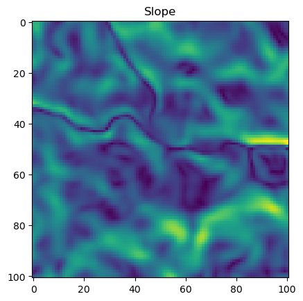
# Get the subset of the slope landscape
slope_subset, origin_x, origin_y = subset_function(slope_landscape_norm, x, y, window_size, raster_transform)
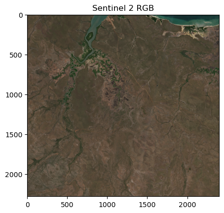
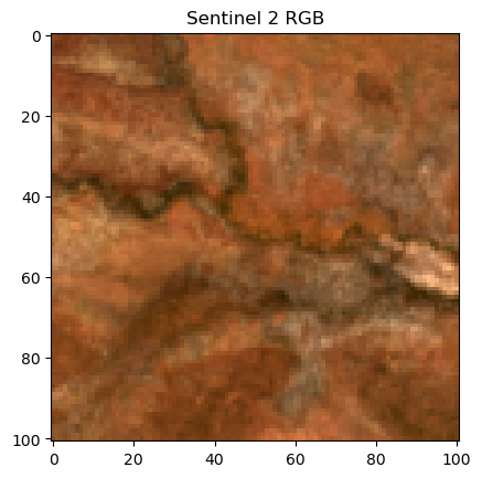
# For sentinel 2 data
selected_month = '2019_01'
# Get the data for the selected month
s2_data = data_dict[selected_month]
# Convert the NumPy array to a PyTorch tensor
s2_tensor = torch.from_numpy(s2_data)
s2_tensor = s2_tensor.float() # Ensure the tensor is of type float
print(s2_tensor.shape) # [bands, height, width]
# Get the subset of the Sentinel-2 bands
s2_b1_subset, origin_x, origin_y = subset_function(s2_tensor[0,:,:], x, y, window_size, raster_transform)
s2_b2_subset, origin_x, origin_y = subset_function(s2_tensor[1,:,:], x, y, window_size, raster_transform)
s2_b3_subset, origin_x, origin_y = subset_function(s2_tensor[2,:,:], x, y, window_size, raster_transform)
s2_b4_subset, origin_x, origin_y = subset_function(s2_tensor[3,:,:], x, y, window_size, raster_transform)
s2_b5_subset, origin_x, origin_y = subset_function(s2_tensor[4,:,:], x, y, window_size, raster_transform)
s2_b6_subset, origin_x, origin_y = subset_function(s2_tensor[5,:,:], x, y, window_size, raster_transform)
s2_b7_subset, origin_x, origin_y = subset_function(s2_tensor[6,:,:], x, y, window_size, raster_transform)
s2_b8_subset, origin_x, origin_y = subset_function(s2_tensor[7,:,:], x, y, window_size, raster_transform)
s2_b8a_subset, origin_x, origin_y = subset_function(s2_tensor[8,:,:], x, y, window_size, raster_transform)
s2_b9_subset, origin_x, origin_y = subset_function(s2_tensor[9,:,:], x, y, window_size, raster_transform)
s2_b11_subset, origin_x, origin_y = subset_function(s2_tensor[10,:,:], x, y, window_size, raster_transform)
s2_b12_subset, origin_x, origin_y = subset_function(s2_tensor[11,:,:], x, y, window_size, raster_transform)
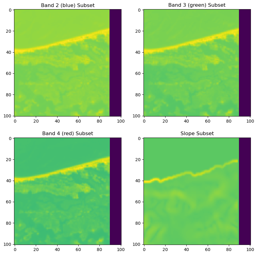
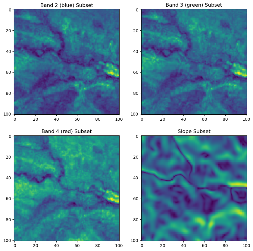
# Plot the subset
fig, axs = plt.subplots(2, 2, figsize=(10, 10))
axs[0, 0].imshow(s2_b2_subset.detach().numpy(), cmap='viridis')
axs[0, 0].set_title('Band 2 (blue) Subset')
axs[0, 1].imshow(s2_b3_subset.detach().numpy(), cmap='viridis')
axs[0, 1].set_title('Band 3 (green) Subset')
axs[1, 0].imshow(s2_b4_subset.detach().numpy(), cmap='viridis')
axs[1, 0].set_title('Band 4 (red) Subset')
axs[1, 1].imshow(slope_subset.detach().numpy(), cmap='viridis')
axs[1, 1].set_title('Slope Subset')