This is where we are generating simulations from the deepSSF model.
Simulating from the deepSSF model is a straightforward process. It requires selecting a starting location, hour of the day and day of the year (the bearing is usually randomly initialised). The local environmental covariates are cropped out as grids with 101 x 101 cells centred on the starting location, and the time inputs are decomposed into their respective sine and cosine components and converted to spatial layers.
The trained model then processes the stack of spatial inputs, resulting in a next-step probability surface, which is exponentiated and sampled with respect to the probability weights. The sampled location is then the next step, and the process is repeated until the desired number of locations is reached.
Import packages
Code
# If using Google Colab, uncomment the following line# !pip install rasterioimport sysprint(sys.version) # Print Python version in useimport numpy as np # Array operationsimport matplotlib.pyplot as plt # Plotting libraryimport torch # Main PyTorch libraryimport os # Operating system utilitiesimport pandas as pd # Data manipulationimport rasterio # Geospatial raster dataimport folium # Interactive mapsfrom datetime import datetime, timedelta # Date/time utilitiesfrom pyproj import Transformer # Coordinate transformationfrom rasterio.plot import show # Plot raster data import deepSSF_model # Import the .py file containing the deepSSF model # Get today's datetoday_date = datetime.today().strftime('%Y-%m-%d')
3.12.5 | packaged by Anaconda, Inc. | (main, Sep 12 2024, 18:18:29) [MSC v.1929 64 bit (AMD64)]
Import the GPS data
We only use this for selecting a spatial extent for the area we want to predict over.
Code
# select the id of that data that the model was trained onbuffalo_id =2005n_samples =10297# 2005 has 10297 samples# Specify the path to your CSV filecsv_file_path =f'../buffalo_local_data_id/buffalo_{buffalo_id}_data_df_lag_1hr_n{n_samples}.csv'# Read the CSV file into a DataFramebuffalo_df = pd.read_csv(csv_file_path)# Display the first few rows of the DataFrameprint(buffalo_df.head())
Instead of importing the stacks of local layers (one for each step), here we want to import the spatial covariates for the extent we want to simulate over. We use an extent that covers all of the observed locations, which refer to as the ‘landscape’.
NDVI
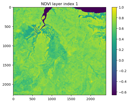
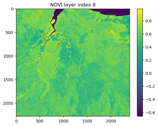
We have monthly NDVI layers for 2018 and 2019, which we import as a stack. The files don’t import with a time component, so we will use a function further down that indexes them correctly.
Code
# for monthly NDVIfile_path ='../mapping/cropped rasters/ndvi_monthly.tif'# read the raster filewith rasterio.open(file_path) as src:# Read the raster band as separate variable ndvi_landscape = src.read([i for i inrange(1, src.count +1)])# Get the metadata of the raster ndvi_meta = src.meta raster_transform = src.transform# Print the metadata to check for time componentprint("Metadata:", ndvi_meta)# Check for specific time-related metadataif'TIFFTAG_DATETIME'in src.tags():print("Time component found:", src.tags()['TIFFTAG_DATETIME'])else:print("No explicit time component found in metadata.")# the rasters don't contain a time component, so we will use a function later to index the layers correctly
Metadata: {'driver': 'GTiff', 'dtype': 'float32', 'nodata': nan, 'width': 2400, 'height': 2280, 'count': 24, 'crs': CRS.from_wkt('LOCAL_CS["GDA94 / Geoscience Australia Lambert",UNIT["metre",1,AUTHORITY["EPSG","9001"]],AXIS["Easting",EAST],AXIS["Northing",NORTH]]'), 'transform': Affine(25.0, 0.0, 0.0,
       0.0, -25.0, -1406000.0)}
No explicit time component found in metadata.
Prepare the NDVI data
There are a few things we need to do to prepare the landscape layers.
First, we need to ensure that there are no NA values in the data. For NDVI we will replace any NA values with -1 (which denotes water), as in our case that is typically why they were set to NA.
Secondly, the model expects the covariates to on the same scale as the training data. We will therefore scale the NDVI data using the same max and min scaling parameters as the training data. To get these, there are some min and max print statements in the deepSSF_train.ipynb script. When we plot the NDVI data below we will see that the values will no longer range from 0 to 1, which is because there are values in the landscape layers that are outside of the range of the training data.
Code
# Check the coordinate reference systemprint("NDVI metadata:")print(ndvi_meta)print("\n")# Have a look at the affine transformation parameters that are used to convert pixel # coordinates to geographic coordinates and vice versaprint("Affine transformation parameters:")print(raster_transform)print("\n")# Check the shape (layers, row, columns) of the rasterprint("Shape of the raster:")print(ndvi_landscape.shape)# Replace NaNs in the original array with -1, which represents waterndvi_landscape = np.nan_to_num(ndvi_landscape, nan=-1.0)# from the stack of local layers (training data)ndvi_max =0.8220ndvi_min =-0.2772# Convert the numpy array to a PyTorch tensorndvi_landscape_tens = torch.from_numpy(ndvi_landscape)# Normalizing the datandvi_landscape_norm = (ndvi_landscape_tens - ndvi_min) / (ndvi_max - ndvi_min)# Show two example layers of the scaled NDVI datalayer_index =1plt.imshow(ndvi_landscape_norm[layer_index,:,:].numpy())plt.colorbar() plt.title(f'NDVI layer index {layer_index}')plt.show()layer_index =8plt.imshow(ndvi_landscape_norm[layer_index,:,:].numpy())plt.colorbar() plt.title(f'NDVI layer index {layer_index}')plt.show()
# Path to the canopy cover raster filefile_path ='../mapping/cropped rasters/canopy_cover.tif'# read the raster filewith rasterio.open(file_path) as src:# Read the raster band as separate variable canopy_landscape = src.read(1)# Get the metadata of the raster canopy_meta = src.meta
Prepare the canopy cover data
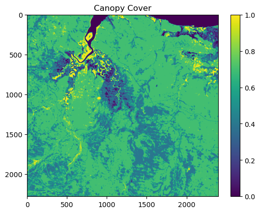
As with the NDVI data, we need to ensure that there are no NA values in the data.
As the canopy cover values in the landscape layer are within the same range as the training data, we see that the values range from 0 to 1.
Code
# Check the canopy metadata:print("Canopy metadata:")print(canopy_meta)print("\n")# Check the shape (rows, columns) of the canopy raster:print("Shape of canopy raster:")print(canopy_landscape.shape)print("\n")# Check for NA values in the canopy raster:print("Number of NA values in the canopy raster:")print(np.isnan(canopy_landscape).sum())# Define the maximum and minimum canopy values from the stack of local layers:canopy_max =82.5000canopy_min =0.0# Convert the canopy data from a NumPy array to a PyTorch tensor:canopy_landscape_tens = torch.from_numpy(canopy_landscape)# Normalise the canopy data:canopy_landscape_norm = (canopy_landscape_tens - canopy_min) / (canopy_max - canopy_min)# Visualise the normalised canopy cover:plt.imshow(canopy_landscape_norm.numpy())plt.colorbar()plt.title('Canopy Cover')plt.show()
Canopy metadata:
{'driver': 'GTiff', 'dtype': 'float32', 'nodata': -3.3999999521443642e+38, 'width': 2400, 'height': 2280, 'count': 1, 'crs': CRS.from_wkt('LOCAL_CS["GDA94 / Geoscience Australia Lambert",UNIT["metre",1,AUTHORITY["EPSG","9001"]],AXIS["Easting",EAST],AXIS["Northing",NORTH]]'), 'transform': Affine(25.0, 0.0, 0.0,
       0.0, -25.0, -1406000.0)}


Shape of canopy raster:
(2280, 2400)


Number of NA values in the canopy raster:
0
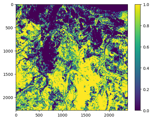
Herbaceous vegetation
Code
# Path to the herbaceous vegetation raster filefile_path ='../mapping/cropped rasters/veg_herby.tif'# read the raster filewith rasterio.open(file_path) as src:# Read the raster band as separate variable herby_landscape = src.read(1)# Get the metadata of the raster herby_meta = src.meta
Code
# Check the herbaceous metadata:print("Herbaceous metadata:")print(herby_meta)print("\n")# Check the shape (rows, columns) of the herbaceous raster:print("Shape of herbaceous raster:")print(herby_landscape.shape)print("\n")# Check for NA values in the herby raster:print("Number of NA values in the herbaceous vegetation raster:")print(np.isnan(herby_landscape).sum())# Define the maximum and minimum herbaceous values from the stack of local layers:herby_max =1.0herby_min =0.0# Convert the herbaceous data from a NumPy array to a PyTorch tensor:herby_landscape_tens = torch.from_numpy(herby_landscape)# Normalize the herbaceous data:herby_landscape_norm = (herby_landscape_tens - herby_min) / (herby_max - herby_min)# Visualize the normalised herbaceous cover:plt.imshow(herby_landscape_norm.numpy())plt.colorbar()plt.show()
Herbaceous metadata:
{'driver': 'GTiff', 'dtype': 'float32', 'nodata': -3.3999999521443642e+38, 'width': 2400, 'height': 2280, 'count': 1, 'crs': CRS.from_wkt('LOCAL_CS["GDA94 / Geoscience Australia Lambert",UNIT["metre",1,AUTHORITY["EPSG","9001"]],AXIS["Easting",EAST],AXIS["Northing",NORTH]]'), 'transform': Affine(25.0, 0.0, 0.0,
       0.0, -25.0, -1406000.0)}


Shape of herbaceous raster:
(2280, 2400)


Number of NA values in the herbaceous vegetation raster:
0
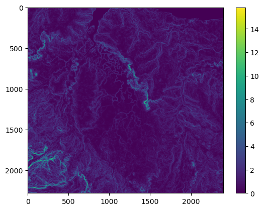
Slope
Code
# Path to the slope raster filefile_path ='../mapping/cropped rasters/slope.tif'# read the raster filewith rasterio.open(file_path) as src:# Read the raster band as separate variable slope_landscape = src.read(1)# Get the metadata of the raster slope_meta = src.meta
Code
# Check the slope metadata:print("Slope metadata:")print(slope_meta)print("\n")# Check the shape (rows, columns) of the slope landscape raster:print("Shape of slope landscape raster:")print(slope_landscape.shape)print("\n")# Check for NA values in the slope raster:print("Number of NA values in the slope raster:")print(np.isnan(slope_landscape).sum())# Replace NaNs in the slope array with 0.0:slope_landscape = np.nan_to_num(slope_landscape, nan=0.0)# Define the maximum and minimum slope values from the stack of local layers:slope_max =12.2981slope_min =0.0006# Convert the slope landscape data from a NumPy array to a PyTorch tensor:slope_landscape_tens = torch.from_numpy(slope_landscape)# Normalize the slope landscape data:slope_landscape_norm = (slope_landscape_tens - slope_min) / (slope_max - slope_min)# Visualize the slope landscape (note: displaying the original tensor, not the normalised data):plt.imshow(slope_landscape_tens.numpy())plt.colorbar()plt.show()
Slope metadata:
{'driver': 'GTiff', 'dtype': 'float32', 'nodata': nan, 'width': 2400, 'height': 2280, 'count': 1, 'crs': CRS.from_wkt('LOCAL_CS["GDA94 / Geoscience Australia Lambert",UNIT["metre",1,AUTHORITY["EPSG","9001"]],AXIS["Easting",EAST],AXIS["Northing",NORTH]]'), 'transform': Affine(25.0, 0.0, 0.0,
       0.0, -25.0, -1406000.0)}


Shape of slope landscape raster:
(2280, 2400)


Number of NA values in the slope raster:
9356
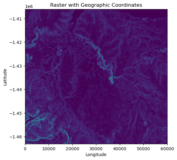
Convert between numpy array and raster
To check that we can go back and forth between numpy arrays (with pixel coordinates) and rasters (with geographic coordinates), we will convert the slope numpy array to a raster.
Code
# Create a figure and axis with matplotlibfig, ax = plt.subplots(figsize=(6, 6))# Convert the slope_landcape (numpy array) to a raster and plot with the rasterio libraryrasterio.plot.show(slope_landscape, transform=raster_transform, ax=ax, cmap='viridis')# Set the title and labelsax.set_title('Raster with Geographic Coordinates')ax.set_xlabel('Longitude')ax.set_ylabel('Latitude')# Show the plotplt.show()
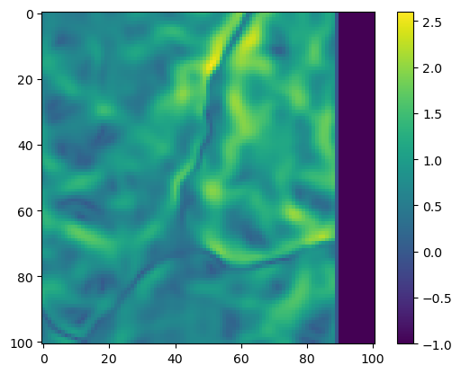
Subset function (with padding)
Now that we have our landscape layers imported, we need a way to crop out the local layers that can be fed into the deepSSF model as covariates.
Also, if our simulated individual goes off the edge of the landscape, we need to pad the landscape layers, in this case we will use values of -1 (which corresponds to water for NDVI and should be avoided) as the deepSSF model can’t handle NA values.
We’ll pick a location near the edge to illustrate this.
Code
# Define geographic coordinates (x: easting/longitude, y: northing/latitude) near the edgex, y =4.912e4, -1.447352e6print(x, y)# Convert geographic coordinates to pixel coordinates using the inverse transformpx, py =~raster_transform * (x, y)# Output the computed pixel coordinatesprint(px, py)# Floor the pixel coordinates to the get the pixel that the location is within.px, py =int(np.floor(px)), int(np.floor(py))# Round the pixel coordinates to the get the pixel that the location is within.# px, py = int(np.round(px)), int(np.round(py))# Ceiling the pixel coordinates to the get the pixel that the location is within.# px, py = int(np.ceil(px)), int(np.ceil(py))# Output the computed pixel coordinatesprint(px, py)
Crop out the local layer, and pad with 0s if necessary.
Code
window_size =101# Define the size of the local covariates (should be the same as the model input size)# Calculate half the window size for centering # (the double slash // is integer or floor division, which rounds down to the nearest whole number)half_window = window_size //2# Determine the starting and ending indices of the window around the centre point (py, px)row_start = py - half_windowrow_stop = py + half_window +1# add one back on to offset the floor divisioncol_start = px - half_windowcol_stop = px + half_window +1# add one back on to offset the floor division# Create an array for the windowed subset, initialised with -1subset = np.full((window_size, window_size), -1, dtype=slope_landscape.dtype)# Find the valid region within the original array boundariesvalid_row_start =max(0, row_start)valid_row_stop =min(slope_landscape.shape[0], row_stop)valid_col_start =max(0, col_start)valid_col_stop =min(slope_landscape.shape[1], col_stop)# Calculate where this valid region maps into the subset arraysubset_row_start = valid_row_start - row_startsubset_row_stop = subset_row_start + (valid_row_stop - valid_row_start)subset_col_start = valid_col_start - col_startsubset_col_stop = subset_col_start + (valid_col_stop - valid_col_start)# Copy the valid part of the raster into the corresponding region of the subset arraysubset[subset_row_start:subset_row_stop, subset_col_start:subset_col_stop] =\ slope_landscape[valid_row_start:valid_row_stop, valid_col_start:valid_col_stop]
Plot the local layer (of slope) in pixel coordinates, which will be 101 x 101 pixels.
Try with different coordinates above to crop out different local layers. Only the centre location is required, which is always the current location of the individual (and we are using the model to predict the next step).
Code
# plot the subsetplt.imshow(subset, cmap='viridis')plt.colorbar()plt.show()
Subset function
Turn the subset code into a function for using in the simulations, although here we are operating on Pytorch tensors rather than numpy arrays, as that is what Pytorch uses.
We have saved this function in the deepSSF_utils.py script for use in other scripts.
Code
def subset_raster_with_padding_torch(raster_tensor, x, y, window_size, transform):# Convert geographic coordinates to pixel coordinates using the inverse transform. px, py =~transform * (x, y)# Floor the pixel coordinates to the get the pixel that the location is within. px, py =int(np.floor(px)), int(np.floor(py))# Round the pixel coordinates to the get the pixel that the location is within.# px, py = int(np.round(px)), int(np.round(py))# Ceiling the pixel coordinates to the get the pixel that the location is within.# px, py = int(np.ceil(px)), int(np.ceil(py))# Compute half the window size to determine the extent around the central pixel. half_window = window_size //2# Determine the boundaries of the window centred on the pixel coordinates. row_start = py - half_window row_stop = py + half_window +1 col_start = px - half_window col_stop = px + half_window +1# Initialise a tensor for the subset with a padding value of -1.0. subset = torch.full((window_size, window_size), -1.0, dtype=raster_tensor.dtype)# Determine the valid region of the raster that falls within the window boundaries. valid_row_start =max(0, row_start) valid_row_stop =min(raster_tensor.shape[0], row_stop) valid_col_start =max(0, col_start) valid_col_stop =min(raster_tensor.shape[1], col_stop)# Calculate the corresponding region within the subset tensor. subset_row_start = valid_row_start - row_start subset_row_stop = subset_row_start + (valid_row_stop - valid_row_start) subset_col_start = valid_col_start - col_start subset_col_stop = subset_col_start + (valid_col_stop - valid_col_start)# Copy the valid region from the raster tensor into the appropriate section of the subset tensor. subset[subset_row_start:subset_row_stop, subset_col_start:subset_col_stop] =\ raster_tensor[valid_row_start:valid_row_stop, valid_col_start:valid_col_stop]# Return the subset along with the starting column and row indices of the window.return subset, col_start, row_start
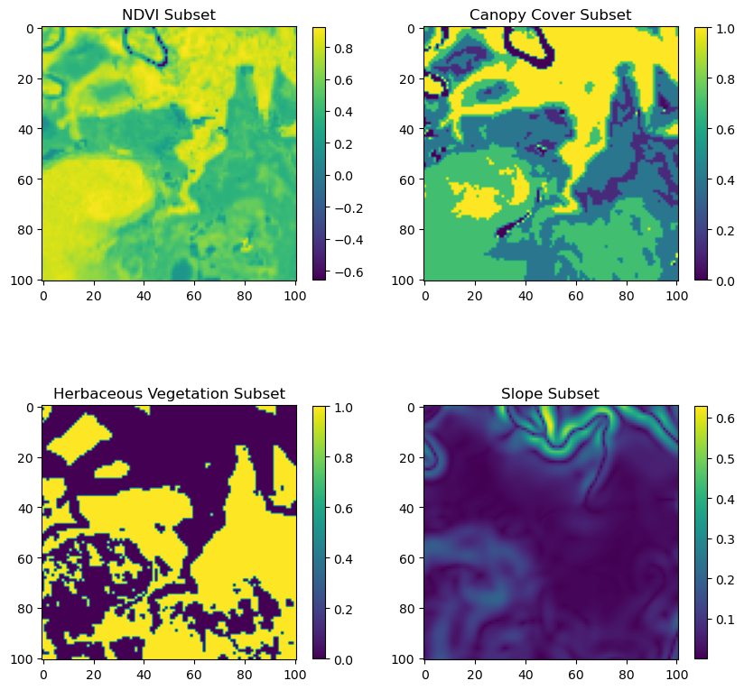
Testing the subset function
Use the subset function to crop out the local layers for all covariates. Try different locations using the x and y coordinates, which are in geographic coordinates (x = easting/longitude, y = northing/latitude).
Code
x =5.8132e4# Set the easting coordinatey =-1.425333e6# Set the northing coordinatewindow_size =101# Define the size of the window to extractwhich_ndvi =1# Select the NDVI layer index# Extract subsets from various raster layers using the custom function.# Each call centres the window at the specified (x, y) location and applies padding where necessary.ndvi_subset, origin_x, origin_y = subset_raster_with_padding_torch(ndvi_landscape_norm[which_ndvi, :, :], x, y, window_size, raster_transform)canopy_subset, origin_x, origin_y = subset_raster_with_padding_torch(canopy_landscape_norm, x, y, window_size, raster_transform)herby_subset, origin_x, origin_y = subset_raster_with_padding_torch(herby_landscape_norm, x, y, window_size, raster_transform)slope_subset, origin_x, origin_y = subset_raster_with_padding_torch(slope_landscape_norm, x, y, window_size, raster_transform)# Create a 2x2 grid of subplots with a fixed figure size.fig, axs = plt.subplots(2, 2, figsize=(10, 10))# Plot the NDVI subset.im0 = axs[0, 0].imshow(ndvi_subset.numpy(), cmap='viridis')fig.colorbar(im0, ax=axs[0, 0], shrink=0.8)axs[0, 0].set_title('NDVI Subset')# Plot the Canopy Cover subset.im1 = axs[0, 1].imshow(canopy_subset.numpy(), cmap='viridis')fig.colorbar(im1, ax=axs[0, 1], shrink=0.8)axs[0, 1].set_title('Canopy Cover Subset')# Plot the Herbaceous Vegetation subset.im2 = axs[1, 0].imshow(herby_subset.numpy(), cmap='viridis')fig.colorbar(im2, ax=axs[1, 0], shrink=0.8)axs[1, 0].set_title('Herbaceous Vegetation Subset')# Plot the Slope subset.im3 = axs[1, 1].imshow(slope_subset.numpy(), cmap='viridis')fig.colorbar(im3, ax=axs[1, 1], shrink=0.8)axs[1, 1].set_title('Slope Subset')
Text(0.5, 1.0, 'Slope Subset')
Load the model
Set the device for the model
Code
# run on the GPU or on the CPU, if a GPU is not availabledevice = torch.device('cuda') if torch.cuda.is_available() else torch.device('cpu')print(f"Using {device} device")
Using cpu device
Define the parameters for the model
Here we enter the specific parameter values and hyperparameters for the model. These are the values that will be used to instantiate the model.
Code
# Define the parameters for the modelparams_dict = {"batch_size": 32, #number of samples in each batch"image_dim": 101, #number of pixels along the edge of each local patch/image"pixel_size": 25, #number of metres along the edge of a pixel"dim_in_nonspatial_to_grid": 4, #the number of scalar predictors that are converted to a grid and appended to the spatial features"dense_dim_in_nonspatial": 4, #change this to however many other scalar predictors you have (bearing, velocity etc)"dense_dim_hidden": 128, #number of nodes in the hidden layers"dense_dim_in_all": 2500,# + 128, #number of inputs entering the fully connected block once the nonspatial features have been concatenated to the spatial features"input_channels": 4+4, #number of spatial layers in each image + number of scalar layers that are converted to a grid"output_channels": 4, #number of filters to learn"kernel_size": 3, #the size of the 2D moving windows / kernels that are being learned"stride": 1, #the stride used when applying the kernel. This reduces the dimension of the output if set to greater than 1"kernel_size_mp": 2, #the size of the kernel that is used in max pooling operations"stride_mp": 2, #the stride that is used in max pooling operations"padding": 1, #the amount of padding to apply to images prior to applying the 2D convolution"num_movement_params": 12, #number of parameters used to parameterise the movement kernel"dropout": 0.1, #the proportion of nodes that are dropped out in the dropout layers"device": device }
As described in the deepSSF_train.ipynb script, we saved the model definition into a file named deepSSF_model.py. We can instantiate the model by importing the file (which was done when importing other packages) and calling the classes parameter dictionary from that script.
# # load the model weights# print(model.state_dict())model.load_state_dict(torch.load(f'outputs/model_training/id2005_med_4_2025-04-14/checkpoint_deepSSF_buffalo2005.pt', map_location=torch.device('cpu'), weights_only=True))# print(model.state_dict())# model.eval()
<All keys matched successfully>
Setup simulation parameters
To get the simulation running we need a few extra functions.
Firstly, we need to index the NDVI layers correctly, based on the time of the simulated location. We’ll do this by creating a function that takes day of the year of the simulated location and returns the correct index for the NDVI layers.
Recall that Python indexes from 0, so when the month_index is equal to 2 for instance, this will index the third layer, which is for March.
Code
# Create a mapping from day of the year to month indexdef day_to_month_index(day_of_year):# Calculate the year and the day within that year base_date = datetime(2018, 1, 1) # base date for the calculation, which is when the NDVI layers start date = base_date + timedelta(days=int(day_of_year) -1) year_diff = date.year - base_date.year month_index = (date.month -1) + (year_diff *12) # month index (0-based, accounting for year change)return month_indexyday =70# day of the year, which is March 11thmonth_index = day_to_month_index(yday)print(month_index)
2
Stack the covariate subset layers
For testing the model.
Code
# Stack the channels along a new axissubset_stack = torch.stack([ndvi_subset, canopy_subset, herby_subset, slope_subset], dim=0)x1 = subset_stackx1 = x1.unsqueeze(0)print(x1.shape)
torch.Size([1, 4, 101, 101])
Additional data
We also need to provide the model with the temporal covariates (hour of day and the day of the year). We will do that by creating a vector of length n_steps for each of these.
For the bearing we will initialise a vector of 0s, but when the model is run we will update the bearings based on the predicted steps. We will then use the bearing of the last step to predict the bearing of the next step (by estimating the turning angle as a deviation from that bearing).
We’ll only index a single time step when testing the function below, but we’ll create the vectors for illustration.
Code
# Define the number of simulation steps.n_steps =100# Create an hour-of-day sequence and repeat it until it reaches n_steps.hour_t2 = np.resize(range(24), n_steps)# Convert hour-of-day values into sine and cosine components.hour_t2_sin = np.sin(2* np.pi * hour_t2 /24)hour_t2_cos = np.cos(2* np.pi * hour_t2 /24)# Create a day-of-year sequence (each day repeated 24 times) and resize to n_steps.yday_sequence = np.repeat(range(yday, 365), 24)yday_t2 = np.resize(yday_sequence, n_steps)# Convert day-of-year values into sine and cosine components.yday_t2_sin = np.sin(2* np.pi * yday_t2 /365)yday_t2_cos = np.cos(2* np.pi * yday_t2 /365)# Initialise a bearing vector with zeroes for all simulation steps, # which will be updated during the simulation.bearing = np.repeat(0., n_steps)# Convert the arrays to PyTorch tensors.hour_t2_tensor = torch.tensor(hour_t2).float()hour_t2_sin_tensor = torch.tensor(hour_t2_sin).float()hour_t2_cos_tensor = torch.tensor(hour_t2_cos).float()yday_t2_tensor = torch.tensor(yday_t2).float()yday_t2_sin_tensor = torch.tensor(yday_t2_sin).float()yday_t2_cos_tensor = torch.tensor(yday_t2_cos).float()bearing = torch.tensor(bearing).float()# Stack the sine and cosine tensors along a new dimension to form the temporal feature tensor.x2_full = torch.stack((hour_t2_sin_tensor, hour_t2_cos_tensor, yday_t2_sin_tensor, yday_t2_cos_tensor), dim=1)# Print the shape of the tensor: (number of steps, number of features).print(x2_full.shape)# Display the temporal features for a specific time step (e.g. index 59).print(f'Temporal information for a single step: {x2_full[59, :]}')
torch.Size([100, 4])
Temporal information for a single step: tensor([ 0.2588, -0.9659,  0.9456,  0.3253])
Functions to recover the hour and yday
Occasionally we will want to recover the hour and day of the year from the sine and cosine terms, so we create a few helper functions to do this.
We have saved these functions in the deepSSF_utils.py script for use in other scripts.
Now we have the covariates ready, we can test the model on them.
Code
# Select a specific time step to test the model, # which just indexes the temporal features in this casestep =17# Run the model with the selected input tensors# Create some extra dimensions to match the model input shapetest = model((x1, x2_full[step,:].unsqueeze(0), bearing[step].unsqueeze(0).unsqueeze(0)))print(test.shape)
torch.Size([1, 101, 101, 2])
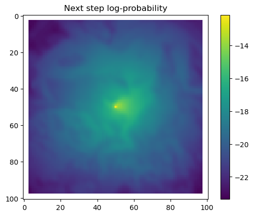
View the model output
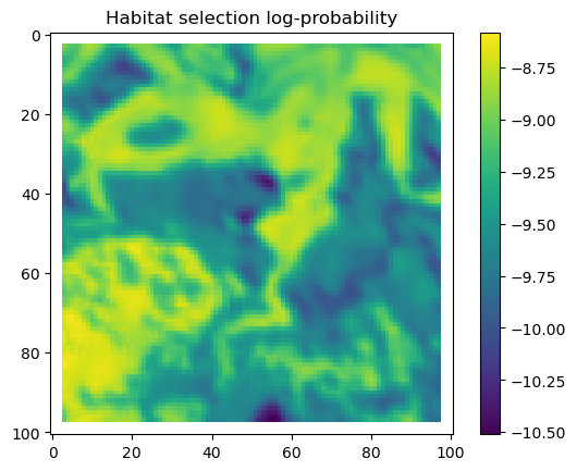
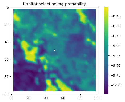
We first check what the hour and yday values were that were inputted to the model, and then plot the habitat selection, movement and next-step predictions from the model.
As convolution filters produce artifacts at the edges of the image, we will crop the habitat selection predictions to remove these. We do this as those edge values are often quite different to the rest of the prediction outputs and change the colour scale, and we only do this when plotting the habitat selection and next-step predictions.
We will also crop out the padding we added to the landscape layers at the edges of the landscape covariates. This we also do during the simulation, as we don’t want cells outside the extent of the landscape to be selected as the next step, i.e., we create a ‘hard’ or ‘reflective’ boundary.
Code
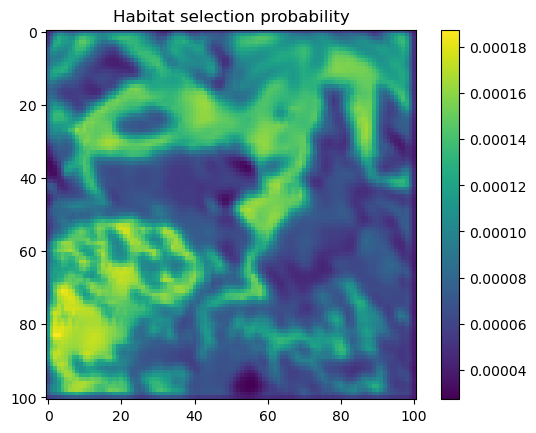
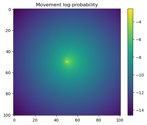
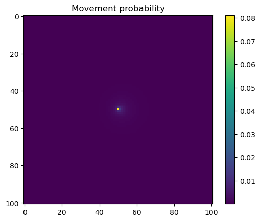
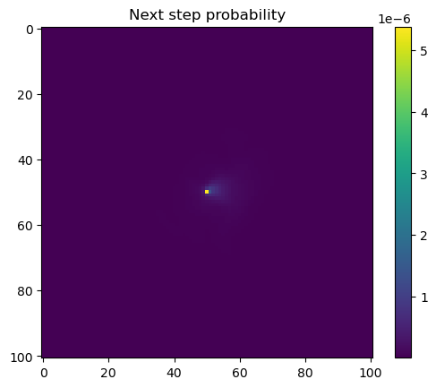
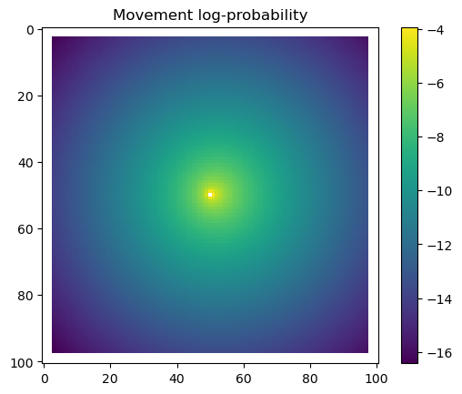
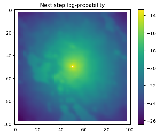
# Extract the temporal features for the specified step and convert to a NumPy array.x2_step = x2_full[step, :].detach().numpy()# Unpack the sine and cosine components for both hour and day-of-year.hour_t2_sin, hour_t2_cos, yday_t2_sin, yday_t2_cos = x2_step# Recover and print the hour value for the step using the sine and cosine components.hour_t2 = recover_hour(hour_t2_sin, hour_t2_cos)print(f'The hour of the step is {round(hour_t2)}')# Recover and print the day-of-year value for the step using the sine and cosine components.yday_t2 = recover_yday(yday_t2_sin, yday_t2_cos)print(f'The day of the year of the step is {round(yday_t2)}')# Extract model predictions from the output tensor.# hab_density: predicted habitat density; move_density: predicted movement density.hab_density = test.detach().numpy()[0, :, :, 0] # habitat densitymove_density = test.detach().numpy()[0, :, :, 1] # movement density# Compute the next step probability by summing habitat and movement densities.next_step = hab_density + move_density# Create border masks for the x and y coordinates to control the colour scale.x_mask = np.ones_like(hab_density)y_mask = np.ones_like(hab_density)# Mask out the edge cells by setting them to negative infinity.x_mask[:, :3] =-np.infx_mask[:, 98:] =-np.infy_mask[:3, :] =-np.infy_mask[98:, :] =-np.inf# Create an edge mask using the NDVI subset as a template.# Replace padding values (-1) with NaN so they do not affect visualisation or sampling.extent_mask = ndvi_subsetextent_mask = torch.where(extent_mask ==-1, torch.tensor(float('nan')), 1).numpy()# Apply the masks to the probability surfaceshab_density = hab_density * extent_maskmove_density = move_density * extent_masknext_step = next_step * extent_mask# Plot the habitat selection log-probability after applying the border and edge masks.plt.imshow(hab_density * x_mask * y_mask)plt.colorbar()plt.title('Habitat selection log-probability')plt.show()# Plot the habitat selection probabilityplt.imshow(np.exp(hab_density))plt.colorbar()plt.title('Habitat selection probability')plt.show()# Plot the movement log-probabilityplt.imshow(move_density)plt.colorbar()plt.title('Movement log-probability')plt.show()# Plot the movement probabilityplt.imshow(np.exp(move_density))plt.colorbar()plt.title('Movement probability')plt.show()# Plot the next step log-probability with the masks applied.plt.imshow(next_step * x_mask * y_mask)plt.colorbar()plt.title('Next step log-probability')plt.show()# Plot the next step probability.plt.imshow(np.exp(next_step))plt.colorbar()plt.title('Next step probability')plt.show()
The hour of the step is 17
The day of the year of the step is 70
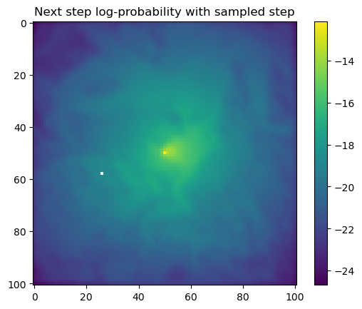
Sample from the probability surface
I.e., choose the individual’s next step
Code
# sample from the array valuesnext_step_exp = np.exp(next_step)# replace NaNs with 0 (which have no probability of being selected)next_step_exp = np.nan_to_num(next_step_exp, nan=0.)# normalise the array to sum to 1next_step_exp = next_step_exp/np.sum(next_step_exp)print(f'Sum of probability values: {np.sum(next_step_exp)}') # should be 1# Flatten the probability surface into a vector (1D array)flat_prob_surface = next_step_exp.flatten()# print(flat_prob_surface)# Generate the corresponding cell indices for the flattened arrayindices = np.arange(flat_prob_surface.size)# print(indices)# Sample from the flattened probability surfacesampled_index = np.random.choice(indices, p=flat_prob_surface)# print(sampled_index)# Print the probability of the sampled indexprint(f'Sampled probability values: {flat_prob_surface[sampled_index]}')# Convert the sampled index back to 2D coordinatessampled_coordinates = np.unravel_index(sampled_index, next_step_exp.shape)print(f'Sampled coordinates: {sampled_coordinates}')# Create a copy of the next step probability surfaces for plotting# The log-probability surface is used for visualisation as it's more informativestep_log_prob = next_step.copy()# The probability surface is used for sampling, but it's not as visually informative# step_log_prob = next_step_exp.copy()# Set the pixel of the next step, which is at (x, y) to -infstep_log_prob[sampled_coordinates] =-np.inf# Plot the next step log-probability with the sampled step highlightedplt.imshow(step_log_prob)plt.colorbar()plt.title('Next step log-probability with sampled step')plt.show()
Sum of probability values:      1.0
Sampled probability values:     0.0004462577865375546
Sampled coordinates:            (33, 51)
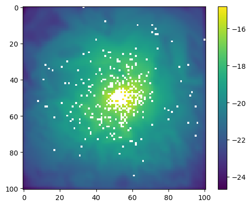
Sample a number of next steps
To get an idea of the distribution of next-steps (from the same starting location), we can loop over the sampling process and block out the selected steps.
Code
for i inrange(100):# Sample from the flattened probability surface sampled_index = np.random.choice(indices, p=flat_prob_surface)# Convert the sampled index back to 2D coordinates sampled_coordinates = np.unravel_index(sampled_index, next_step_exp.shape)# Set the pixel of the next step, which is at (x, y) to -inf step_log_prob[sampled_coordinates] =-np.infplt.imshow(step_log_prob)plt.colorbar()plt.show()
Return sampled point to geographic coordinates
When simulating, we don’t want to just the pixel values (as they are in reference to the local layer), but we want to return the geographic coordinates of the next step and store those.
Code
print(f'Starting location in geographic coordinates: {x ,y}')print(f'Starting location in landscape layer pixel coordinates: {px, py}')print(f'Sampled next step location (local layer pixel coordinates): {sampled_coordinates}')print(f'landscape pixel locations at the origin of the local layer: {row_start, col_start}')# Add the sampled coordinates to the landscape pixel locations at the origin of the local layer# THE Y COORDINATE (row) COMES FIRSTnew_px = origin_x + sampled_coordinates[1]new_py = origin_y + sampled_coordinates[0]print(f'landscape pixel coordinates of the sampled next step: {new_px, new_py}')# Convert landscape pixel coordinates to geographic coordinatesnew_x, new_y = raster_transform * (new_px, new_py)print(f'Landscape geograhic coordinates at the next step: {new_x, new_y}')
Starting location in geographic coordinates:                 (31500.0, -1430000.0)
Starting location in landscape layer pixel coordinates:      (52, 52)
Sampled next step location (local layer pixel coordinates):  (48, 55)
landscape pixel locations at the origin of the local layer:  (1604, 1914)
landscape pixel coordinates of the sampled next step:        (2330, 771)
Landscape geograhic coordinates at the next step:            (58250.0, -1425275.0)
Next-step function
Now we have all of the pieces working, we can put them together into function that predicts the next step of the simulated individual. We can then loop over the function to create trajectories.
The next-step function will take the following inputs: - environmental rasters at the landscape level, - the scalar covariates to be turned into grids (temporal covariates in our case), - the previous bearing to predict the turning angle from, - the size of the local layer to crop out, - the current location of the simulated individual, - the raster transformation to convert between pixel and geographic coordinates.
Adding jitter to the next step
As location of the next step is a particular cell (which are 25 m x 25 m), we also have an additional component in the function that adds an element of randomness to where in the cell the next step is. This prevents the location of the next step from being in exactly the same location as the current step (which would lead to a null bearing and 0 step length), and prevents an artificial grid-like pattern from emerging in the simulated trajectories. As all of the probability values are exactly the same within a cell, this is analogous to the process of simulating from an SSF, where continuous step lengths and turning angles are drawn from their distributions, which land somewhere in a particular cell. However, the difference is that the probability values for the movement kernel in an SSF are still continuous, whereas in the deepSSF model they are discrete (due to calculating the movement probability for each cell). This may lead to artifacts for steps very close to the current location, as the Gamma distribution has high probability near 0.
We ‘jitter’ the point by adding a small amount of noise in the x and y direction. This small amount is drawn from a 2D (uncorrelated) normal distribution with a mean of 0 and a standard deviation of 6.5 m, such that about 95% of the jittered points will fall within the 25 m x 25 m cell. If the jittered point falls outside of the cell, we re-sample the jittered point until it falls within the cell.
This could have also been a uniform distribution between -12.5 and 12.5 in the x and y directions, but we chose a normal distribution as for the centre cell we still want it to be close to 0. This was a modelling choice and different choices here will have slightly different effects (although mainly on the step length and turning angle distributions). The cell that was selected, which becomes the cell to start the next step from, will be the same.
Code
def simulate_next_step(landscape_raster_tensors, scalars_to_grid, bearing, window_size, x_loc, y_loc, landscape_raster_transform):# Extract subsets from the landscape rasters results = [subset_raster_with_padding_torch(raster_tensor, x=x_loc, y=y_loc, window_size=window_size, transform=landscape_raster_transform) for raster_tensor in landscape_raster_tensors]# Unpacking the results subset_rasters_tensors, origin_xs, origin_ys =zip(*results)# print(subset_rasters_tensors)# Stack the processed tensors along a new dimension (e.g., dimension 0) x1 = torch.stack(subset_rasters_tensors, dim=0) x1 = x1.unsqueeze(0)# print(x1.shape)# Pull out the NDVI layer to get where is was set to -1 (outside the landscape extent) ndvi_local_layer = x1[0, 0, :, :]# create masking layer to remove outside of the extent mask = torch.where(ndvi_local_layer ==-1, torch.tensor(float('nan')), 1)# Set the scalar values as the x2 model input x2 = scalars_to_grid# Set the bearing values as the x3 model input x3 = bearing test = model((x1, x2, x3))# print(test.shape) # Debugging print - should be (1, 101, 101, 2) hab_log_prob = test[:, :, :, 0] move_log_prob = test[:, :, :, 1] step_log_prob = (hab_log_prob + move_log_prob) step_log_prob = step_log_prob * mask hab_log_prob = hab_log_prob.squeeze() move_log_prob = move_log_prob.squeeze() step_log_prob = step_log_prob.squeeze()# sample from the array values step_prob = torch.exp(step_log_prob) step_prob = torch.nan_to_num(step_prob, nan=0.) step_prob_norm = step_prob/torch.sum(step_prob)# print(torch.sum(step_prob_norm)) # Debugging print - should be 1# Flatten the probability surface flat_step_prob_norm = step_prob_norm.flatten().detach().numpy()# print(flat_prob_surface) # Debugging print# Generate the corresponding indices for the flattened array indices = np.arange(flat_step_prob_norm.size)# Sample from the flattened probability surface sampled_index = np.random.choice(indices, p=flat_step_prob_norm)# Convert the sampled index back to 2D coordinates sampled_coordinates = np.unravel_index(sampled_index, step_prob_norm.shape)# THE Y COORDINATE COMES FIRST in the sampled pixel coordinates new_px = origin_xs[0] + sampled_coordinates[1] new_py = origin_ys[0] + sampled_coordinates[0]# Convert geographic coordinates to pixel coordinates new_x, new_y = raster_transform * (new_px, new_py)# Sample from a normal distribution with mean 0 and sd 6.5, # which are the parameters where the cell contains ~ 95% of density# if it's outside the bounds of the cell, resamplewhileTrue: jitter_x = np.random.normal(12.5, 6.5)if0<= jitter_x <=25:break# Sample jitter for new_y and ensure it is within bounds# The jitter in the y axis is negative because geographic coordinates increase upwards, # whereas pixel coordinates increase downwardswhileTrue: jitter_y = np.random.normal(-12.5, 6.5)if-25<= jitter_y <=0:break# Add the valid jitter to new_x and new_y new_x = new_x + jitter_x new_y = new_y + jitter_y# print(new_x, new_y)# Return the new_x and new_y coordinates, # the probability surfaces for optional plotting,# and the sampled coordinates (next step in local layer pixel coordinates)return new_x, \ new_y, \ hab_log_prob, \ move_log_prob, \ step_log_prob, \ sampled_coordinates[1], \ sampled_coordinates[0]
Test the function
Code
# Choose a location in the landscapex =3.15e4# easting coordinatey =-1.43e6# northing coordinate# Landscape scale rasters - select one of the NDVI layerslandscape_raster_list = [ndvi_landscape_norm[which_ndvi,:,:], canopy_landscape_norm, herby_landscape_norm, slope_landscape_norm]# Select the temporal features for the specific stepx2 = x2_full[3,:].unsqueeze(0)# print(x2.shape)# Select the bearing for the specific stepbearing_step = bearing[3].unsqueeze(0).unsqueeze(0)# print(bearing_step.shape)test_outputs = simulate_next_step(landscape_raster_tensors=landscape_raster_list, scalars_to_grid=x2, bearing=bearing_step, window_size=101, x_loc=x, y_loc=y, landscape_raster_transform=raster_transform)new_x, new_y, hab_log_prob, move_log_prob, step_log_prob, px, py = test_outputsprint(f'New location in local layer pixel coordinates: {px, py}')print(f'New location in geographic coordinates: {new_x, new_y}')# Set the pixel of the next step, which is at (px, py) to -infhab_log_prob[(px, py)] =-np.infmove_log_prob[(px, py)] =-np.infstep_log_prob[(px, py)] =-np.inf# Plot the habitat selection log-probability after applying the border maskplt.imshow(hab_log_prob.detach().numpy()[:,:] * x_mask * y_mask)plt.colorbar()plt.title('Habitat selection log-probability')plt.show()# Plot the movement log-probabilityplt.imshow(move_log_prob.detach().numpy()[:,:] * x_mask * y_mask)plt.colorbar()plt.title('Movement log-probability')plt.show()# Plot the next step log-probability with the masks applied.plt.imshow(step_log_prob.detach().numpy()[:,:] * x_mask * y_mask)plt.colorbar()plt.title('Next step log-probability')plt.show()
New location in local layer pixel coordinates:      (51, 49)
New location in geographic coordinates:             (31530.190943327136, -1429985.6839061948)
Generate trajectory
Now we can loop over the next-step function to generate a trajectory.
Setup parameters
Code
# Setup the simulation parametersn_steps =3000starting_yday =206# starting location, which was the starting location of buffalo 2005 (the training data)start_x =41969.310875start_y =-1.435671e+06# output directory for saving plotsoutput_dir =f'outputs/deepSSF_prob_maps/id{buffalo_id}_{today_date}'os.makedirs(output_dir, exist_ok=True)
Create simulation inputs from the parameters
Create empty lists to store the simulated locations and bearings, and initialise the vectors of temporal covariates.
Code
# Empty lists to store the x and y coordinatesx = np.repeat(0., n_steps)y = np.repeat(0., n_steps)# Set the first entry as the starting locationx[0], y[0] = start_x, start_y# Create an hour-of-day sequence and repeat it until it reaches n_steps.hour_t2 = np.resize(range(24), n_steps)# Convert hour-of-day values into sine and cosine components.hour_t2_sin = np.sin(2* np.pi * hour_t2 /24)hour_t2_cos = np.cos(2* np.pi * hour_t2 /24)# Create the day of the year sequences # We want to index the NDVI layers into next year, which is why the ydays go above 365yday_t2 = np.repeat(range(starting_yday, starting_yday +365), 24)yday_t2 = np.resize(yday_t2, n_steps)# Convert day-of-year values into sine and cosine components.yday_t2_sin = np.sin(2* np.pi * yday_t2 /365)yday_t2_cos = np.cos(2* np.pi * yday_t2 /365)# Initialise a bearing vector with zeroes for all simulation steps, # which will be updated during the simulation.bearing = np.repeat(0., n_steps)# Convert lists to PyTorch tensorshour_t2_tensor = torch.tensor(hour_t2).float()hour_t2_sin_tensor = torch.tensor(hour_t2_sin).float()hour_t2_cos_tensor = torch.tensor(hour_t2_cos).float()yday_t2_tensor = torch.tensor(yday_t2).float()yday_t2_sin_tensor = torch.tensor(yday_t2_sin).float()yday_t2_cos_tensor = torch.tensor(yday_t2_cos).float() bearing_tensor = torch.tensor(bearing).float()# Stack tensors column-wise to create a tensor of shape [n_steps, 4]x2_full = torch.stack((hour_t2_sin_tensor, hour_t2_cos_tensor, yday_t2_sin_tensor, yday_t2_cos_tensor), dim=1)# Initialize variables to cache the previous yday and month indexprevious_yday =None
Trajectory loop
Now we can loop over the next-step function to generate a trajectory. Essentially we have to a some starting location, which goes through the simulate_next_step function to get the next location, which then becomes the current location for the next step.
For indexing, the location we are trying to predict (the next step) is index i, and the current location is index i-1. This prevents the loop from breaking by storing the final location at i+1, which is outside of the loop range.
The bearing at i-1 is the bearing between i-1 and i-2, i.e., the bearing that location i-1 was approached from.
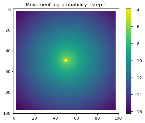
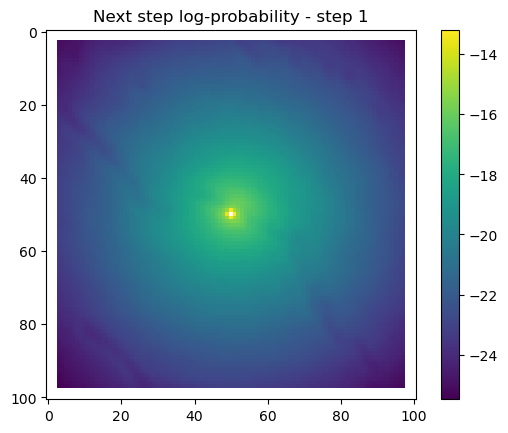
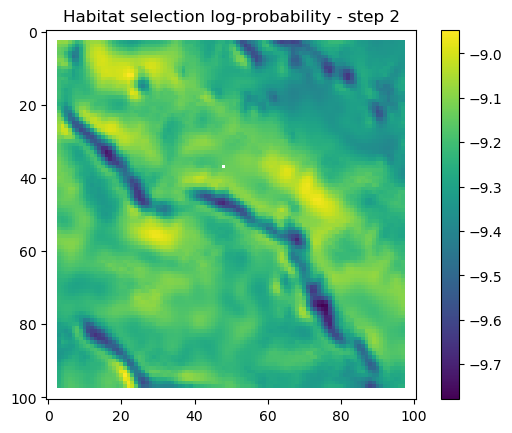
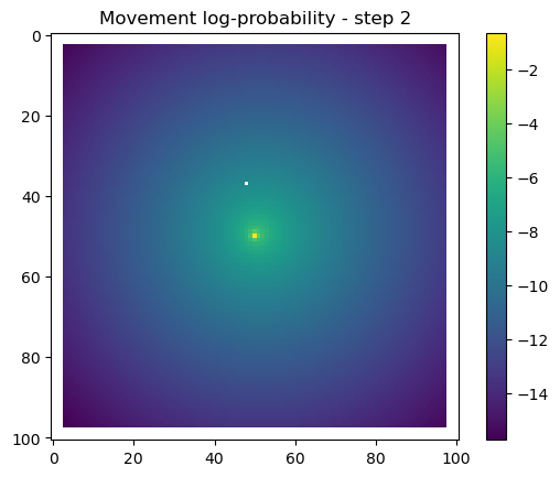
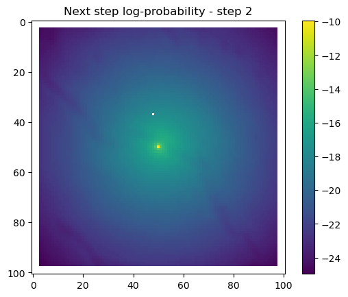
After the simulate_next_step function, we have some code for generating and saving plots of the habitat selection, movement and next-step predictions (all on the log-scale as they’re more informative). This is helpful to check that everything is working as expected, but can also be used for making animations (when plotting the surfaces for the whole trajectory). When making a trajectory it can be helpful to comment out the plt.show() lines, so the plots will just save to file and not pop up.
Code
for i inrange(1, n_steps): x_loc = x[i-1] y_loc = y[i-1]# calculate the bearing from the previous locationif i >1: bearing_rad = np.arctan2(y[i-1] - y[i-2], x[i-1] - x[i-2])# bearing_rad = np.random.uniform(-np.pi, np.pi)else:# if it's the first step, sample a random bearing bearing_rad = np.random.uniform(-np.pi, np.pi)# Store the bearing in the vector bearing[i-1] = bearing_rad# print("Bearing[i-1]", bearing[i-1]) # Debugging print# Convert the bearing to a tensor and add dimensions for the batch and channel bearing_tensor = torch.tensor(bearing[i-1]).unsqueeze(0).unsqueeze(0)# print(bearing_tensor.shape) # Debugging print# Select the temporal features for the specific step x2 = x2_full[i-1,:].unsqueeze(dim=0)# print(x2)# Determine the month index based on the day of the year day_of_year = yday_t2[i-1]if day_of_year != previous_yday: month_index = day_to_month_index(day_of_year) previous_yday = day_of_year# print(f'Day of the year: {day_of_year}') # Debugging print# print(f'Month index: {month_index}') # Debugging print# Select the landscape rasters for the specific month landscape_raster_list = [ndvi_landscape_norm[month_index,:,:], canopy_landscape_norm, herby_landscape_norm, slope_landscape_norm]# Run the simulation function for the next step sim_outputs = simulate_next_step(landscape_raster_tensors=landscape_raster_list, scalars_to_grid=x2, bearing=bearing_tensor, window_size=101, x_loc=x_loc, y_loc=y_loc, landscape_raster_transform=raster_transform)# Unpack the simulation outputs (new_x, new_y, hab_log_prob, move_log_prob, step_log_prob, px, py) = sim_outputs# print(f'New location in pixel coordinates {px, py}') # Debugging print# print(f'New location in geographic coordinates {new_x, new_y}\n') # Debugging print# Store the new x and y coordinates x[i] = new_x y[i] = new_y# -------------------------------------------------------------------------# Plot the probability surfaces for habitat selection, movement, and next step# -------------------------------------------------------------------------# The x_mask and y_mask objects should have already been defined earlier in the code# Plot the first few probability surfaces - change the condition to i < n_steps to plot allif i <3:## Habitat probability surface hab_log_prob = hab_log_prob.detach().numpy()[:,:] * x_mask * y_mask hab_log_prob[py, px] =-np.inf## Movement probability surface move_log_prob = move_log_prob.detach().numpy()[:,:] * x_mask * y_mask move_log_prob[py, px] =-np.inf## Next step probability surface next_step_log = step_log_prob.detach().numpy()[:,:] * x_mask * y_mask next_step_log[py, px] =-np.inf filename_hab =f"{output_dir}/id{buffalo_id}_hab_log_prob_{today_date}_{i}.png" plt.figure() # Create a new figure plt.imshow(hab_log_prob) plt.colorbar() plt.title(f'Habitat selection log-probability - step {i}') plt.draw() # Ensure the plot is rendered plt.savefig(filename_hab, dpi=96) plt.show() plt.close() # Close the figure to free memory filename_move =f"{output_dir}/id{buffalo_id}_move_log_prob_{today_date}_{i}.png" plt.figure() plt.imshow(move_log_prob) plt.colorbar() plt.title(f'Movement log-probability - step {i}') plt.draw() plt.savefig(filename_move, dpi=96) plt.show() plt.close() filename =f"{output_dir}/id{buffalo_id}_next_step_log_{today_date}_{i}.png" plt.figure() plt.imshow(next_step_log) plt.colorbar() plt.title(f'Next step log-probability - step {i}') plt.draw() plt.savefig(filename, dpi=96) plt.show() plt.close()
Example animation of the trajectory
We saved 250 habitat selection, movement and next-step plots, which we can use to make an animation of the trajectory. We can used an online gif maker to do this.
Habitat selection log-probabilities
The daily pattern is quite clear in the habitat selection, as the model is using the hour of the day as a covariate, and learns a representation of the temporal habitat selection patterns.
Next-step log-probabilities
The fine-scale temporal dynamics also come out in the movement dynamics, with an expanding and contracting movement kernel.
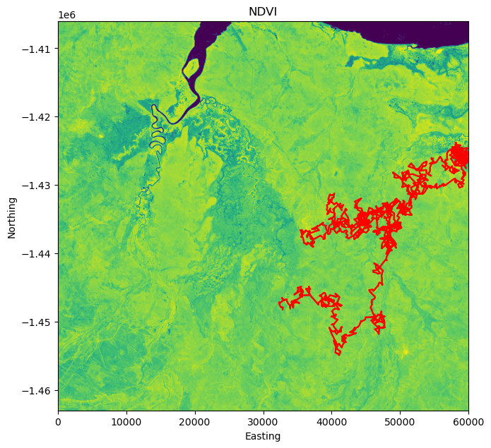
Plot the simulated trajectory
Code
# Create a figure and axis with matplotlibfig, ax = plt.subplots(figsize=(7.5, 7.5))# Plot the NDVI rasterrasterio.plot.show(ndvi_landscape[which_ndvi,:,:], transform=raster_transform, ax=ax, cmap='viridis')# Set the title and labelsax.set_title('NDVI')ax.set_xlabel('Easting')ax.set_ylabel('Northing')# Number of simulated locations (to just get valid points)n_sim_points = np.min([x[x>0].shape[0], y[y<0].shape[0]])print(n_sim_points)# Plot the simulated trajectoryplt.plot(x[1:n_sim_points], y[1:n_sim_points], color ='red')plt.plot(x[1:n_sim_points], y[1:n_sim_points], color ='red')plt.show()
3000
Plot with interactive map
We can also use the folium library to plot the trajectory on an interactive map. This is useful for checking the trajectory in more detail, as we can zoom in and out and pan around the map.
We used the ESRI World Imagery basemap, although other basemaps can be used (check the folium documentation for more options: https://python-visualization.github.io/folium/latest/user_guide/raster_layers/tiles.html).
Code
# ESRI World Imagery basemap tiletiles ='https://server.arcgisonline.com/ArcGIS/rest/services/World_Imagery/MapServer/tile/{z}/{y}/{x}'# Create a folium map with the ESRI World Imagery basemap (centred on starting location)basemap = folium.Map(location=[-12.2995517, 134.3782028], tiles=tiles, attr='Esri', zoom_start =10)
Change projection of the trajectory
We will also reproject the observed data to the same projection as the basemap, so that we can overlay the observed data on the map as well.
We use the pyproj library to reproject the data. We will reproject the observed data to the same projection as the basemap, which is the World Geodetic System 1984 (WGS84) that used latitude and longitute coordinates, denoted by EPSG:4326.
Code
# Create the reprojection functioncoord_transformer = Transformer.from_crs('epsg:3112', 'epsg:4326')# Observed data# Convert the easting and northing coordinates to geographic coordinatesbuffalo_lon, buffalo_lat = coord_transformer.transform(buffalo_df['x_'], buffalo_df['y_'])print(buffalo_lon[1:4], buffalo_lat[1:4])# Create a list of coordinate pairs (rather than separate lists)buffalo_coordinates = [[lon, lat] for lon, lat inzip(buffalo_lon, buffalo_lat)]print(buffalo_coordinates[1:4])# Simulated data# Convert the easting and northing coordinates to geographic coordinatessim_lon, sim_lat = coord_transformer.transform(x[x>0], y[x>0])# Create a list of coordinate pairssim_coordinates = [[lon, lat] for lon, lat inzip(sim_lon, sim_lat)]
# Add the buffalo datafolium.PolyLine( locations=buffalo_coordinates, color='red', weight=2, opacity=1, tooltip='Buffalo trajectory').add_to(basemap)# Add the simulated datafolium.PolyLine( locations=sim_coordinates, color='blue', weight=2, opacity=1, tooltip='Simulated trajectory').add_to(basemap)# Plot the mapbasemap
Make this Notebook Trusted to load map: File -> Trust Notebook
Write the trajectory to a csv
Only run this once otherwise it will create duplicates
Code
# output directory for saving trajectoriesoutput_dir_traj =f'outputs/deepSSF_trajectories/{buffalo_id}'os.makedirs(output_dir_traj, exist_ok=True)# Combine vectors into a DataFrametrajectory_df = pd.DataFrame({'x': x[x>0], 'y': y[x>0], 'hour': hour_t2[x>0], 'yday': yday_t2[x>0], 'bearing': bearing[x>0] })n_steps_actual = x[x>0].shape[0]# Save the DataFrame to a CSV fileindex =1csv_filename =f'{output_dir_traj}/deepSSF_id{buffalo_id}_{n_steps_actual}steps_{index}_{today_date}.csv'# Check if the file already exists and find a new name if necessarywhile os.path.exists(csv_filename): csv_filename =f'{output_dir_traj}/deepSSF_id{buffalo_id}_{n_steps_actual}steps_{index}_{today_date}.csv' index +=1print(csv_filename)trajectory_df.to_csv(csv_filename, index=True)
# -------------------------------------------------------------------------# Setup parameters# -------------------------------------------------------------------------n_trajectories =10n_steps =3000starting_yday =206# -------------------------------------------------------------------------# Looping over simulated individuals# -------------------------------------------------------------------------for j inrange(1, n_trajectories+1):# Empty lists to store the x and y coordinates x = np.repeat(0., n_steps) y = np.repeat(0., n_steps)# Set the first entry as the starting location x[0], y[0] = start_x, start_y# Create sequence of steps step =range(1, n_steps)# Create an hour-of-day sequence and repeat it until it reaches n_steps. hour_t2 = np.resize(range(24), n_steps)# Convert hour-of-day values into sine and cosine components. hour_t2_sin = np.sin(2* np.pi * hour_t2 /24) hour_t2_cos = np.cos(2* np.pi * hour_t2 /24)# Create the day of the year sequences # We want to index the NDVI layers into next year, which is why the ydays go above 365 yday_t2 = np.repeat(range(starting_yday, starting_yday +365), 24) yday_t2 = np.resize(yday_t2, n_steps)# Convert day-of-year values into sine and cosine components. yday_t2_sin = np.sin(2* np.pi * yday_t2 /365) yday_t2_cos = np.cos(2* np.pi * yday_t2 /365)# Initialise a bearing vector with zeroes for all simulation steps, # which will be updated during the simulation. bearing = np.repeat(0., n_steps)# Convert lists to PyTorch tensors hour_t2_tensor = torch.tensor(hour_t2).float() hour_t2_sin_tensor = torch.tensor(hour_t2_sin).float() hour_t2_cos_tensor = torch.tensor(hour_t2_cos).float() yday_t2_tensor = torch.tensor(yday_t2).float() yday_t2_sin_tensor = torch.tensor(yday_t2_sin).float() yday_t2_cos_tensor = torch.tensor(yday_t2_cos).float() bearing_tensor = torch.tensor(bearing).float()# Stack tensors column-wise to create a tensor of shape [n_steps, 4] x2_full = torch.stack((hour_t2_sin_tensor, hour_t2_cos_tensor, yday_t2_sin_tensor, yday_t2_cos_tensor), dim=1)# Initialize variables to cache the previous yday and month index previous_yday =None# -------------------------------------------------------------------------# Simulation loop# -------------------------------------------------------------------------for i inrange(1, n_steps): x_loc = x[i-1] y_loc = y[i-1]# calculate the bearing from the previous locationif i >1: bearing_rad = np.arctan2(y[i-1] - y[i-2], x[i-1] - x[i-2])else:# if it's the first step, sample a random bearing bearing_rad = np.random.uniform(-np.pi, np.pi)# Store the bearing in the vector bearing[i-1] = bearing_rad# print("Bearing[i-1]", bearing[i-1]) # Debugging print# Convert the bearing to a tensor and add dimensions for the batch and channel bearing_tensor = torch.tensor(bearing[i-1]).unsqueeze(0).unsqueeze(0)# print(bearing_tensor.shape) # Debugging print# Select the temporal features for the specific step x2 = x2_full[i-1,:].unsqueeze(dim=0)# print(x2) # Debugging print# Determine the month index based on the day of the year day_of_year = yday_t2[i-1]if day_of_year != previous_yday: month_index = day_to_month_index(day_of_year) previous_yday = day_of_year# print(f'Day of the year: {day_of_year}') # Debugging print# print(f'Month index: {month_index}') # Debugging print# Select the landscape rasters for the specific month landscape_raster_list = [ndvi_landscape_norm[month_index,:,:], canopy_landscape_norm, herby_landscape_norm, slope_landscape_norm]# Run the simulation function for the next step sim_outputs = simulate_next_step(landscape_raster_tensors=landscape_raster_list, scalars_to_grid=x2, bearing=bearing_tensor, window_size=101, x_loc=x_loc, y_loc=y_loc, landscape_raster_transform=raster_transform)# Unpack the simulation outputs new_x, new_y, hab_log_prob, move_log_prob, step_log_prob, px, py = sim_outputs# print(f'New location in pixel coordinates {px, py}') # Debugging print# print(f'New location in geographic coordinates {new_x, new_y}\n') # Debugging print# Store the new x and y coordinates x[i] = new_x y[i] = new_y# -------------------------------------------------------------------------# Save the simulated trajectories# -------------------------------------------------------------------------# save the data frames individually# Combine vectors into a DataFrame trajectory_df = pd.DataFrame({'x': x[x>0], 'y': y[x>0], 'hour': hour_t2[x>0], 'yday': yday_t2[x>0], 'bearing': bearing[x>0]}) n_steps_actual = x[x>0].shape[0]# Save the DataFrame to a CSV file index = j csv_filename =f'{output_dir_traj}/deepSSF_floor_jitter_id{buffalo_id}_{n_steps_actual}steps_{index}_{today_date}.csv'# Check if the file already exists and find a new name if necessarywhile os.path.exists(csv_filename): csv_filename =f'{output_dir_traj}/deepSSF_floor_jitter_id{buffalo_id}_{n_steps_actual}steps_{index}_{today_date}.csv' index +=1print(csv_filename) trajectory_df.to_csv(csv_filename, index=True)