Step Selection Intuition

In this section we hope to provide some intuition for how we set up the deepSSF model the way that we did, and how we simulated from it, such that it is easier to follow the paper and the code. We hope that is is also helpful understanding how to simulate from step selection functions more generally as well.
Animal movement data as steps
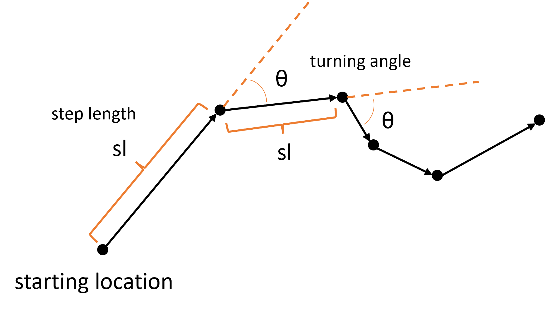
Firstly, when we have animal movement data, we can consider it as a series of steps, each with a step length and a turning angle:
If we aggregate every step across the trajectory (which may be many thousands of steps long), the step lengths and turning angles form distributions:
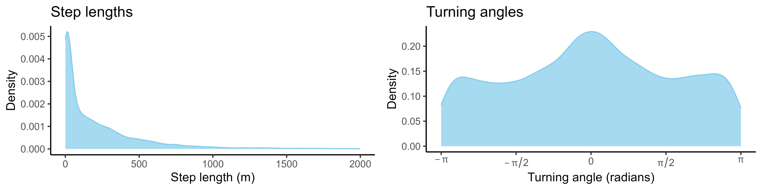
If we wanted to simulate from this movement process, we could simply sample values from these step length and turning angle distributions (either from the observed values or by fitting parametric distributions and sampling from those). This would be a correlated random walk; correlated as it has persistence in some direction, usually in the forward direction.
Movement kernel
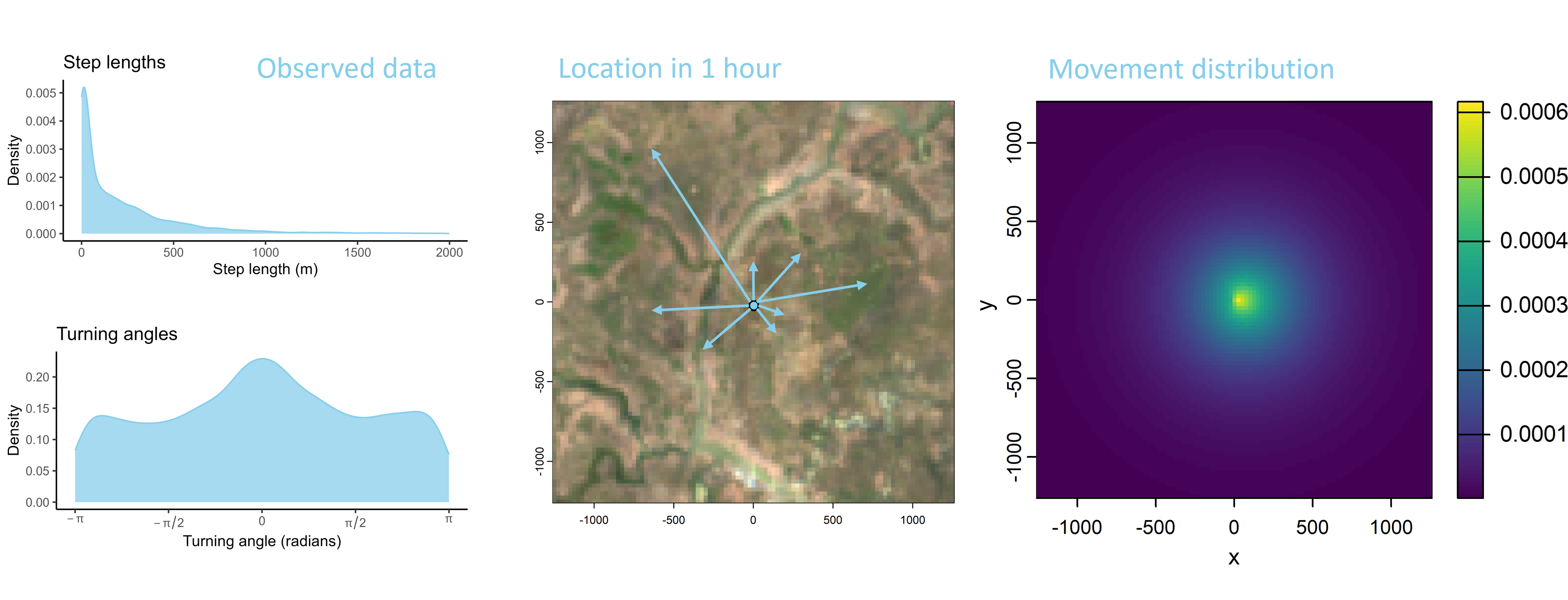
We can also consider the step lengths and turning angles to be a two-dimensional distribution or a ‘movement probability surface’. We could then introduce correlation between the step lengths and the turning angles (i.e. straight turning angles with long steps), giving a more realistic movement kernel. But mainly it is helpful to visualise the movement kernel as a 2D surface, which we can sample our next-steps from.
Habitat selection
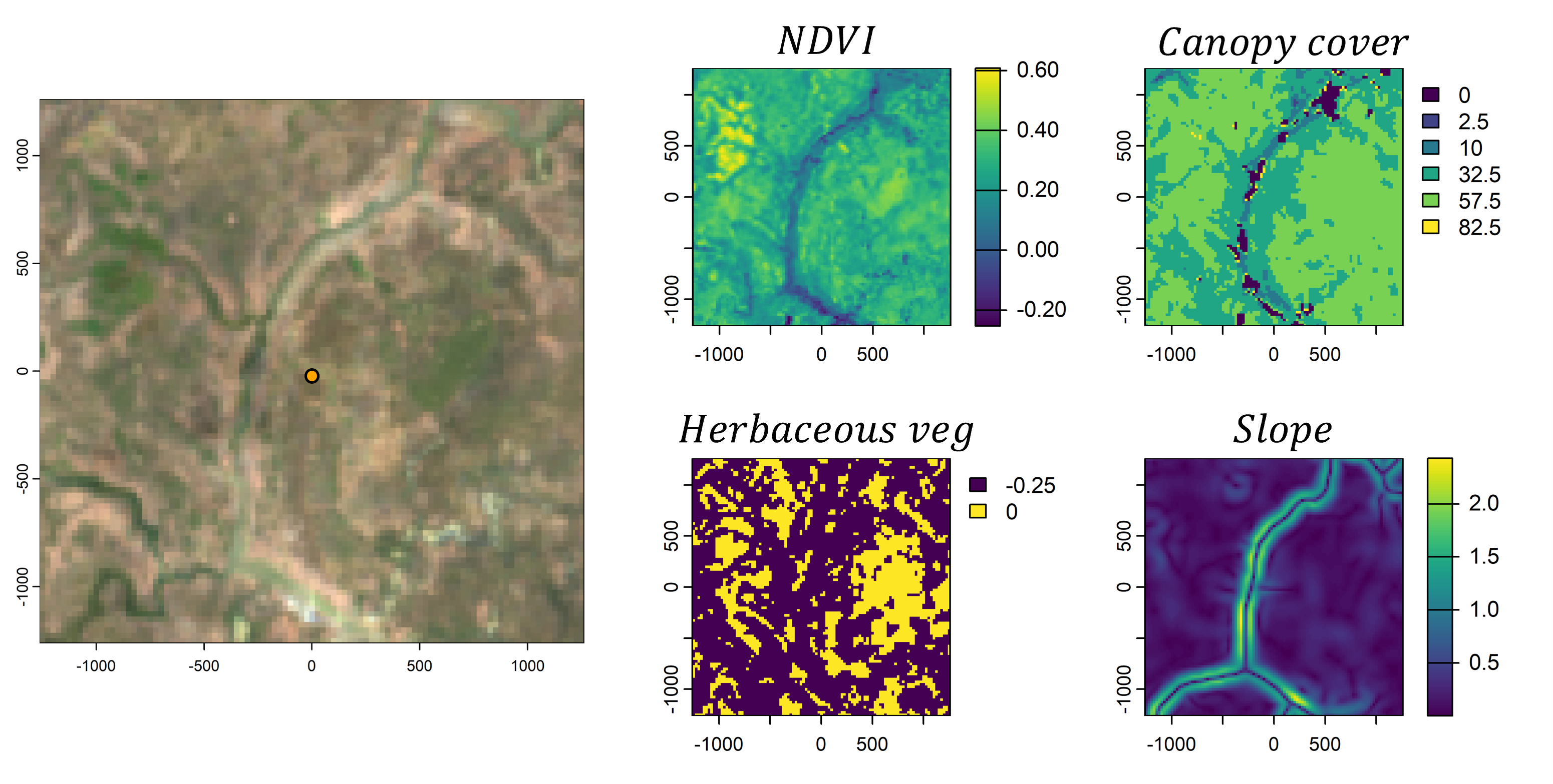
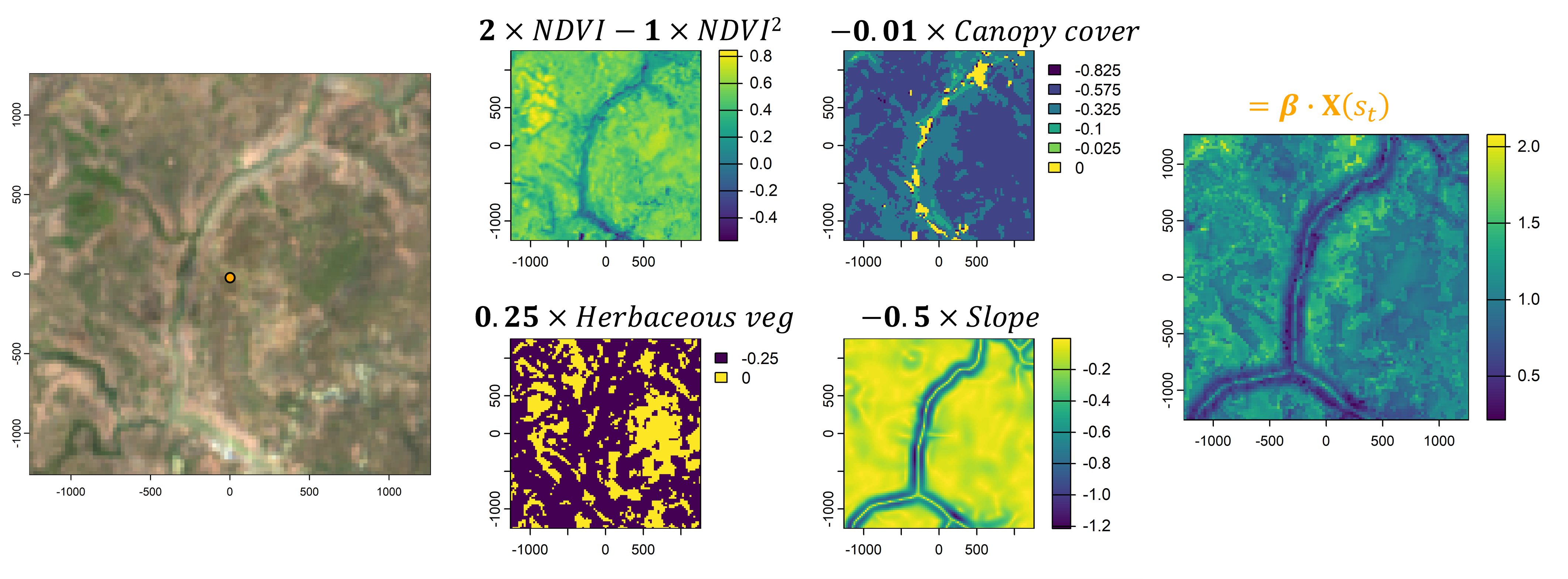
However, animals also respond to environmental features. If we take the local landscape that is within the range of movement (i.e. containing most of the movement kernel’s probability), we can imagine this landscape being comprised of different components, such as the vegetation (described through something like Normalised Difference Vegetation Index - NDVI), how dense the canopy is, or what the terrain is like. We would call these our spatial covariates.
We then need some way to describe or quantify a relationship between the animal and the spatial covariates. One way to do this is by using (log-)linear relationships, where increasing values of the covariate lead to increasing or decreasing selection, or via quadratic relationships which add some more flexibility. These relationships can be encoded in coefficients, which may be positive or negative. If we then sum these outputs together we get a habitat selection (log-)probability surface. Something like this is usually called a resource selection function (shown here on the log-scale and unnormalised).
We now have a movement probability surface and a habitat selection probability surface.
Next-step probability
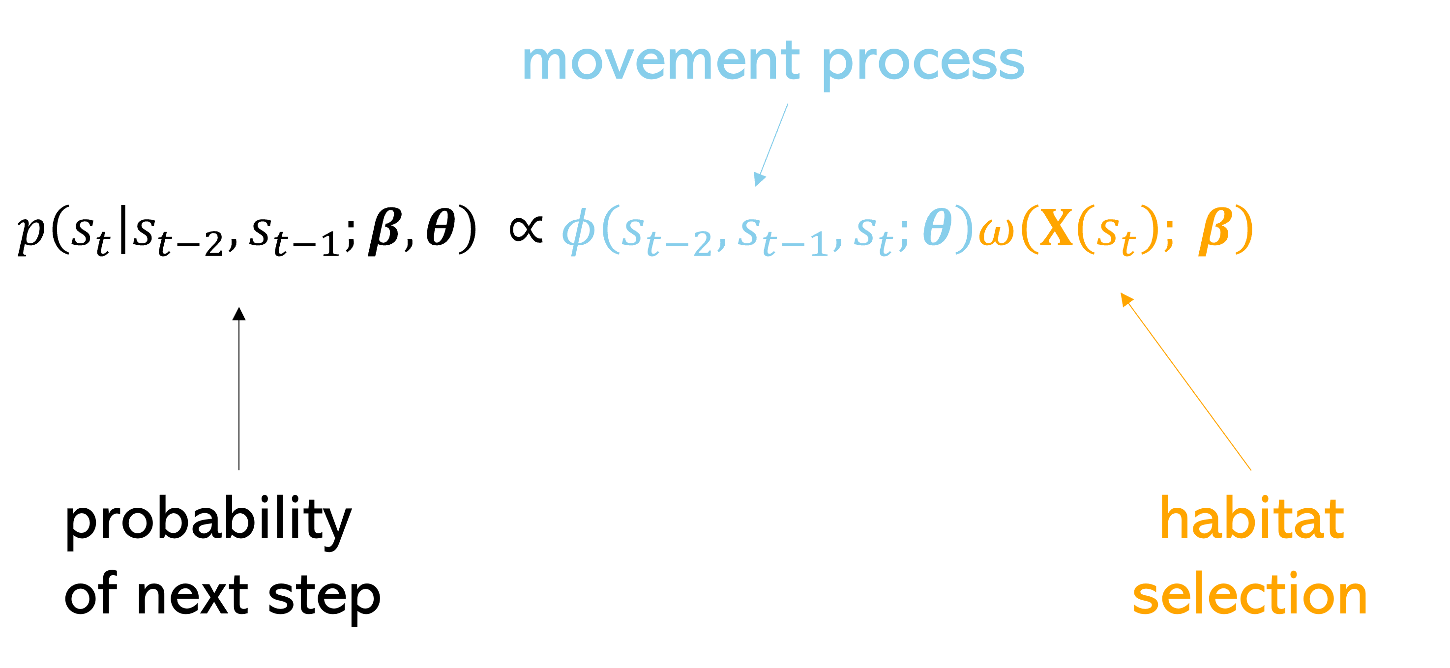
If we then combine those surfaces together (by adding on the log-scale or multiplying on the natural probability scale), we get the probability of the next step that the animal may take, or the next-step probability surface.
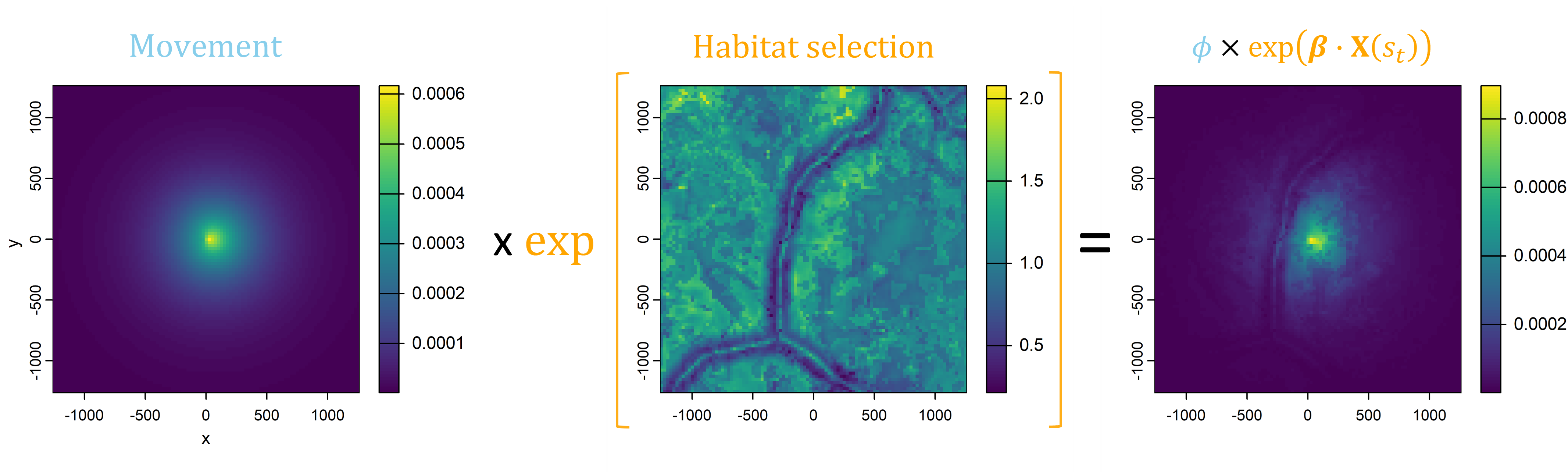
Essentially, we have (simplistically) described a step selection function (SSF), where the probability of selecting the next step is described by a movement process and a habitat selection process.
Note: the movement parameters are typically estimated at the same time as the habitat selection, resulting in movement distributions that would be observed in the absence of any external covariates, also called the ‘selection-free movement kernel’ (Avgar et al. 2016).
Simulating trajectories
Once we have a model with parameters that describe the next-step probability surface, we can easily simulate from it.
We do this by choosing a starting location, generating the next-step probability surface for the local area (centred on the current location), and then selecting the next step from it with respect to the probability weights.
This location then becomes the starting point for the next step, and the process repeats until a trajectory is generated. This forms a biased correlated random walk, as there is bias towards certain habitat, and correlation in the movement process (Duchesne et al. 2015).
Here brighter colours denote higher selection values.
This is all we need for a basic simulation of animal movement that has a movement and a habitat selection process.
Limitations
However, animal movement is complex. The relationship between the animal and the surrounding covariates is unlikely to follow a linear or quadratic relationship, and the animal may not be responding to only the covariate values in particular cells, but to broader habitat features that are described by specific arrangements of cells. The animal’s relationship may also be influenced by interactions between covariates, i.e., NDVI that is selected differently depending on the terrain.
Animal movement is also dynamic across multiple time-scales, such as daily movements that also change across the course of the year. My co-authors and I explored fine-scale temporal dynamics using SSFs in another paper (Forrest et al. 2024), showing that the movement and habitat selection of buffalo changed quite dramatically throughout the day, but having daily selection that also changed across seasons (within the same model) was quite difficult and it would have been hard to estimate the parameters.
Although, a promising approach for including temporal dynamics and interactions of covariates is to use smooth terms in SSFs (Klappstein et al. 2024).
deepSSF
When we formulate the problem in this way, with explicit processes of movement and habitat selection, it starts to become easier to see how we might use different modelling approaches. From the spatial (and temporal) covariates we need to quantify a relationship to the animal’s observed locations, indicating what resources are likely to be selected, and we need to parameterise a movement kernel from the observed data.
We show how we do this in the deepSSF Model Overview tab, where we provide an overview of the deepSSF model in more detail.