Deep Learning Concepts
To help understand how the deepSSF model represents animal movement, we show some deep learning concepts in the context of the deepSSF model. Some parts of these are taken directly from the main text of the paper, and some from the Supplementary Materials, both of which we have expanded here.
There are numerous courses, books and tutorials online that are excellent for getting started with deep learning, many of them free. I’ve provided a couple that I’ve found helpful below, or have been recommended, but there are many, many more.
Additional Resources
Online courses for deep learning
Learn PyTorch for Deep Learning: Zero to Mastery: https://www.learnpytorch.io/ - I found this resource very useful for getting started with deep learning and PyTorch, and it is accompanied by 25 hours of YouTube videos!
PyTorch Tutorials: https://pytorch.org/tutorials/ - Helpful for getting started with PyTorch, although not as detailed as the course above.
DeepLearning.AI Courses and other Resources: https://www.deeplearning.ai/ - I haven’t tried these personally but I have heard they are good.
Excellent videos for developing an intuition about the mechanics of deep learning
3Blue1Brown’s Neural Network YouTube Series: https://youtube.com/playlist?list=PLZHQObOWTQDNU6R1_67000Dx_ZCJB-3pi&si=_v1iHPWA8VeecsP0 - Grant Sanderson’s (creator of the 3Blue1Brown channel) YouTube videos are beautiful and extremely informative, particularly for visualising complex processes such as deep learning. The YouTube series on neural networks include an introduction to neural networks (essentially just the fully-connected layers described below), gradient descent, backpropagation, LLMs and more.
Free books
Dive into Deep Learning: https://d2l.ai/index.html
- Interactive deep learning book with code, math, and discussions
- Implemented with PyTorch, NumPy/MXNet, JAX, and TensorFlow
Understanding Deep Learning: https://udlbook.github.io/udlbook/
- Free PDF download
Probabilistic Machine Learning: An Introduction: https://probml.github.io/pml-book/book1.html
- This ‘introduction’ is still over 800 pages long, but the ‘ProbML’ book is an introduction to probabilistic machine learning more generally, which includes probability theory, statistics theory, regression models and more, before getting into deep learning. It’s quite a mathematical entry, but it clearly highlights the links between typical statistical models and techniques with deep learning models, such as neural networks.
- Click the download draft button for a copy
Convolutional Layers
A convolutional layer applies a series of learned convolution filters across the spatial dimensions of the input, producing feature maps that highlight important patterns or structures. This operation preserves spatial hierarchies within the data and allows the network to capture local dependencies. The processing elements of convolutional layers are therefore the convolution filters.
Helpful resources for convolutional layers
CNN explainer: An interactive visualisation of convolution filters and activation functions
Animated AI: Animations over depth (for when we have multiple channels, such as different spatial layers)
https://hannibunny.github.io/mlbook/neuralnetworks/convolutionDemos.html: 2D animations (i.e., for a single channel)
Convolution filters
A convolution filter, also called a kernel, is a small, learned matrix (in our case they were 3 cells x 3 cells) that sweeps across a set of spatial inputs and applies element-wise operations to the input data. Through training, the filter adapts to capture specific features, such as edges or textures, from localised regions of the input. Each filter is optimised via backpropagation to extract important features from the spatial layers. For the deepSSF models the convolution filters give probability to habitat features that are associated with observed buffalo locations.
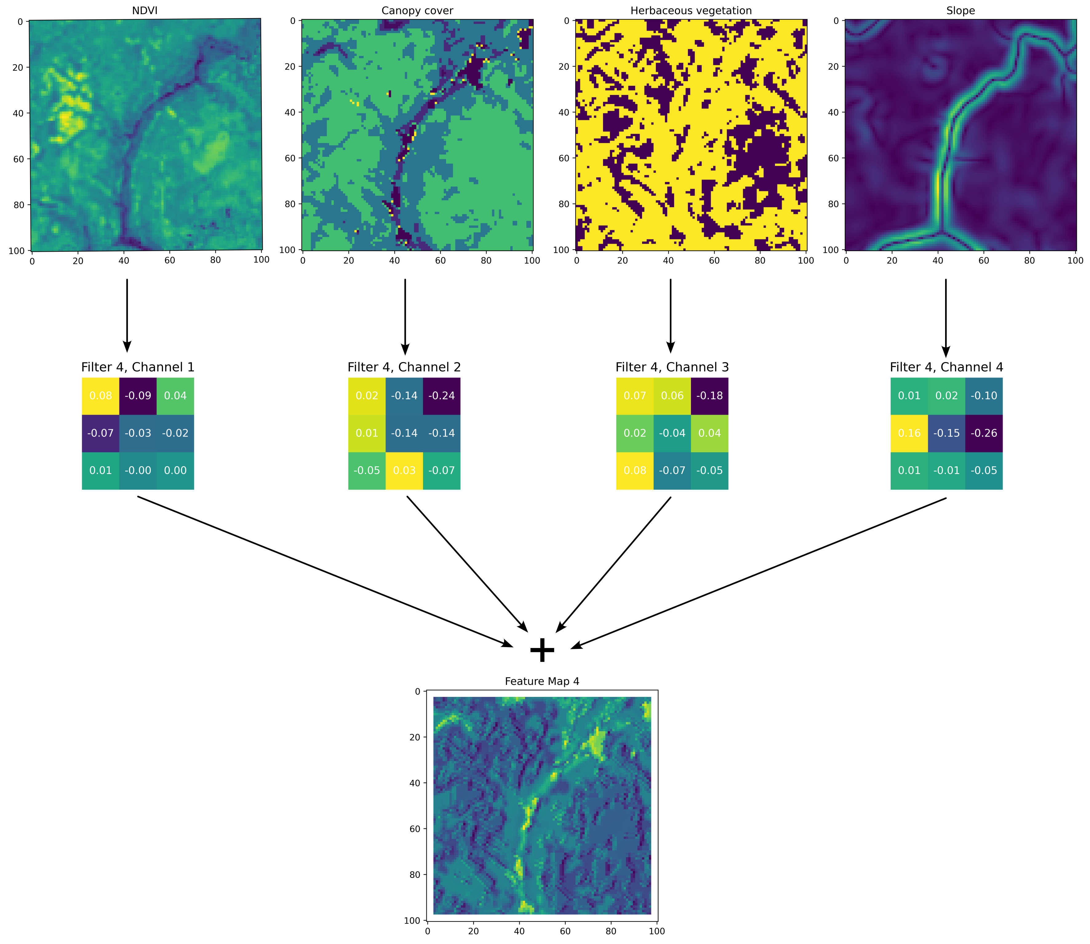
Here we show a single convolution filter from the habitat selection network and the resulting feature map (prior to being processed by an activation function, which in our case was the ReLU). A single convolution filter has \(n\) channels that relate to the \(n\) channels of the input layers, and each filter channel convolves over its respective input layer, which are then added together to create the feature map for that filter.

To understand the convolution process, imagine the convolution filter channel starting in the top left corner of the spatial input, say NDVI, with the central cell of the filter in the top left corner. For each cell, the value of NDVI will be multiplied by the corresponding cell in the filter channel, resulting in nine values, which are then summed together to form the top left cell in the intermediate feature map (which are not shown here). The filter then moves to the right by one cell (as the stride is equal to one), and the element-wise multiplication is repeated. This results in transformations of many small, overlapping windows across the spatial input, resulting in another layer (the intermediate feature map).
This process is repeated for the next input layer, which has its own filter channel, until each input layer has been processed into an intermediate feature map. These intermediate feature maps are then summed to create the output feature map for that filter. During training it is the values of the convolution filters that are updated. It can be helpful to see this process animated, and an example of an animation of a convolution filter across multiple channels can be found at: https://animatedai.github.io/. In the linked animation, the inputs are \(7 \times 6 \times 8\), and each coloured block in the middle represents a \(3 \times 3 \times 8\) filter, and in total there are 8 filters. Each coloured layer in the output to the right represents a feature map. Note that there is no padding for these operations, which results in a dimension reduction, but below there is an animation is shown with padding which retains the \(d \times d\) dimensions of the inputs, such that we have used in our deepSSF model.
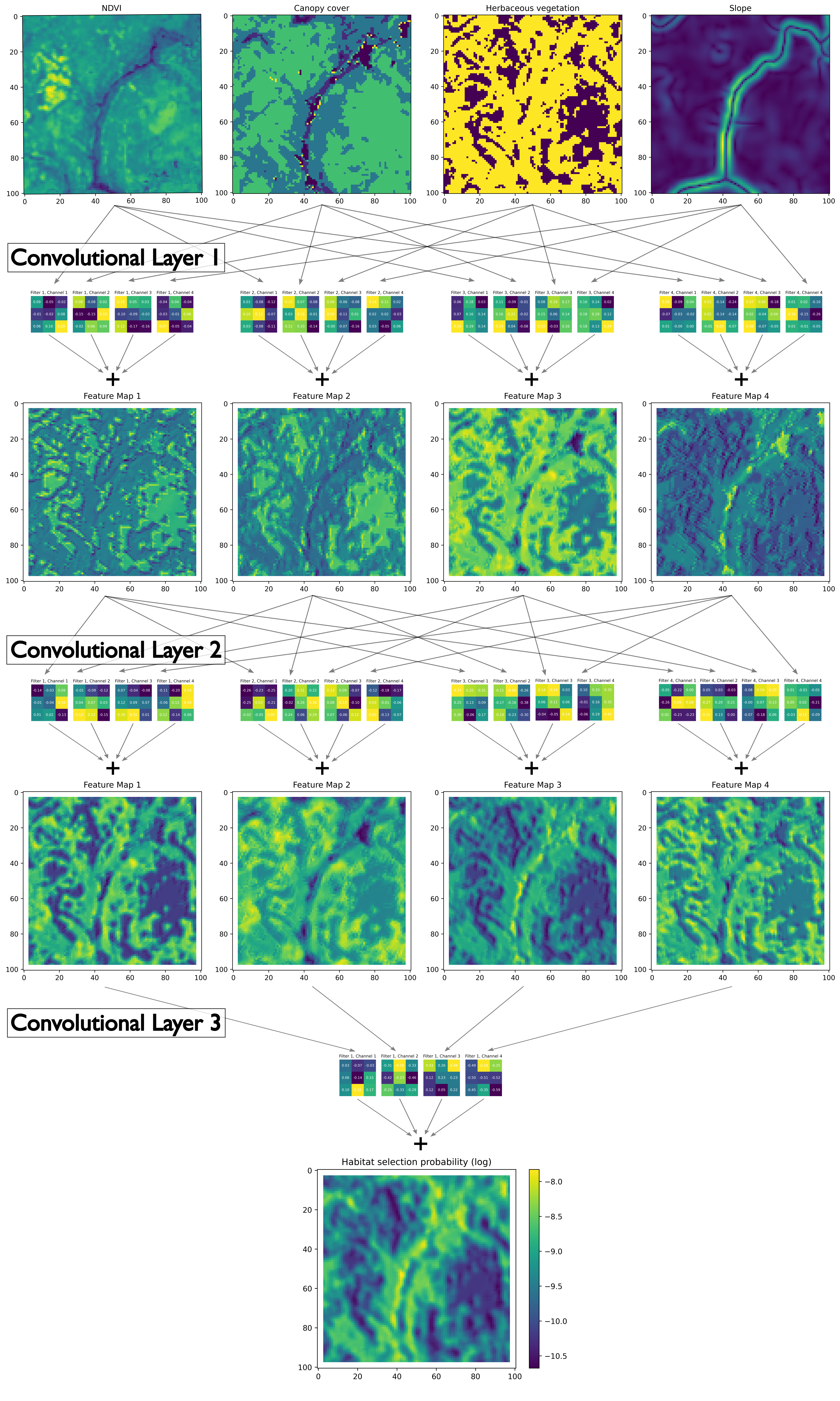
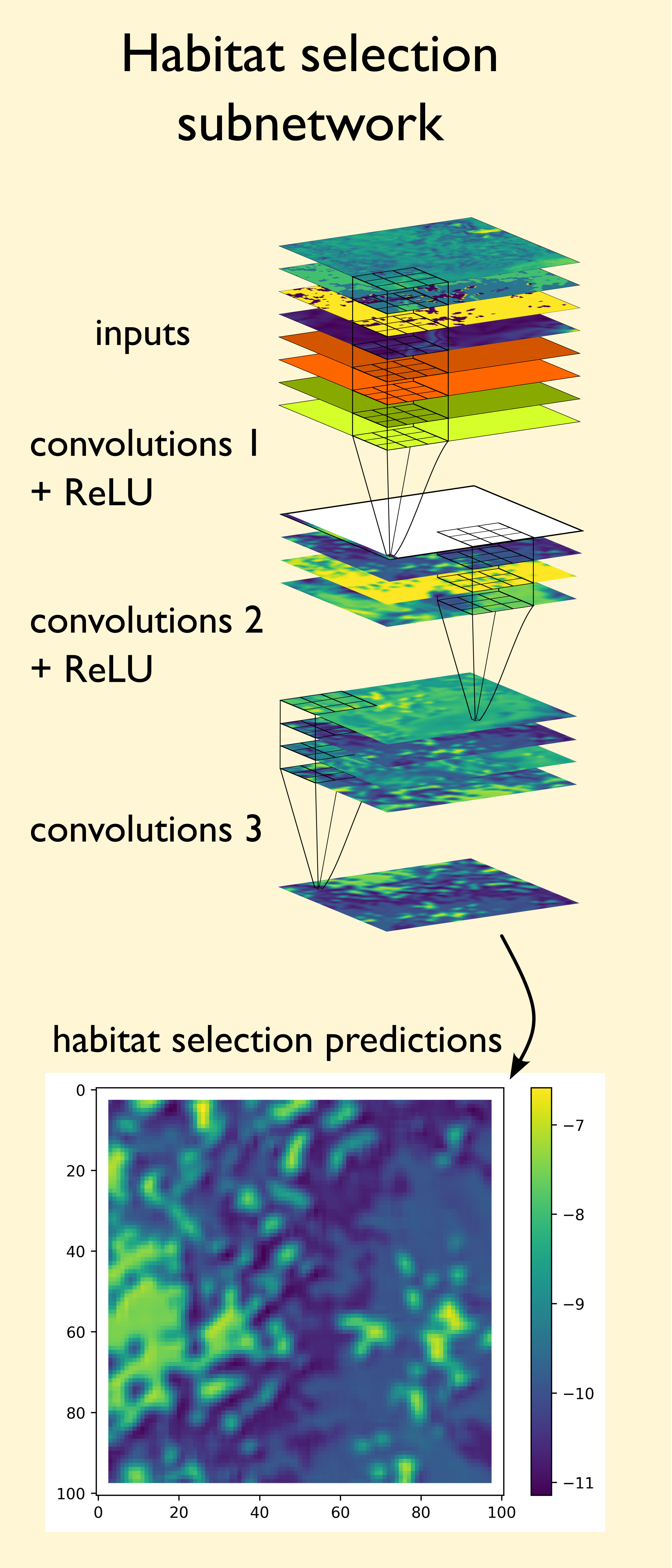
The benefits of deep learning come from many small operations combining together to represent complex and abstract processes. Here we show all of the convolutional layers that were used in the habitat selection subnetwork, except that for clarity we do not show the temporal inputs (hour of the day and day of the year decomposed into sine and cosine terms), which are also converted to spatial inputs, as shown in Figure 1 in the main text. Each convolution filter has a channel for each of the spatial inputs and produces a single feature map.
In Convolution Layer 1 there are four filters, resulting in four feature maps, which each extract different aspects and features of the inputs (i.e. transform them in different ways). In Convolutional Layer 2 there are also four filters, except that the inputs to this layer are the feature maps outputted by Convolutional Layer 1. Convolutional Layer 3 then takes the feature maps from Convolutional Layer 2 as inputs and processes and aggregates them into a single feature map, which are the log probabilities of the habitat selection subnetwork (there is no ReLU after this layer meaning that there can be values less than zero - which are exponentiated values below 1). The successive convolutional layers are what give deep learning their name, where ‘depth’ is described by the number of successive processing layers, allowing for the models to learn a representation for abstract features in the input covariates.

We can see in the habitat selection subnetwork, we are simply passing the inputs, which are spatial covariates (e.g. NDVI, slope, etc) and temporal covariates which have been turned into grids (see Model Overview), through several convolutional layers which result in the next-step probabilities. During training, the model learns to give probability weight to features (certain values, spatial features) that are associated with the buffalo’s next steps. Thaat means that if there is an observed next step near a river, the model will use the convolution filters to give higher values to the cells in the spatial covariates that describe the river. This could be just the values of the covariates themselves, such as low canopy cover, or it could be the shape of the river described by the arrangement of pixels. As convolution layers assess the local neighbourhood of cells (with a perception that increases as the layers get deeper), they can learn to associate spatial features, such as rivers, waterholes, forest edges, roads, with higher or lower probabilities of being selected as the next step.

The Math
The convolutional layers employed in our neural network architecture are also known as two-dimensional convolutional layers. Two-dimensional convolutional layers provide a mechanism to learn new features or variables of predictive value from gridded data using sets of convolutional weights that are re-used at different locations over two-dimensional space. The input to a two-dimensional convolutional layer is a three-dimensional input tensor, \(\mathbf{Q}\), with dimensions \((d, d, n)\). In the context of our application, \(\mathbf{Q}\) represents a stack of \(n\) spatial covariates in a \(d \times d\) pixel region of habitat surrounding an individual, which in our case was 101 x 101 cells with 25 m x 25 m resolution. Each of the \(n\) spatial covariates (i.e., NDVI, slope, etc.), is usually referred to as a ‘channel’.
The convolutional layer transforms this stack of spatial layers into a new three-dimensional tensor, \(\mathbf{O}\), with dimensions \((d, d, F)\) through the application of \(F\) unique convolution filters (also called kernels) that are learned in neural network training. As convolution layers can be considered to transform the inputs covariates and ‘extract features’ from them, the resulting layers denoted by \(F\) are often called ‘feature maps’ (see Figures below). Each filter can be represented as a \((2w + 1) \times (2w + 1) \times n\) tensor of weights and we denote the collection of these filters as \(\mathbf{W}^{(1)}, \dots, \mathbf{W}^{(F)}\).
The hyper-parameters \(w\) (the spatial width and height in pixels of the filter) and \(F\) are user-specified, and in our application were set as \(w = 1\) and \(F = 4\) in all cases except in the final convolutional layer that had \(F = 1\) to aggregate the preceding feature maps into the final habitat selection map. For \(w = 1\), each filter can be thought of as consisting of \(n\) convolution filters of dimension \(3 \times 3\). Applying filter \(f \in \{ 1, \dots, F \}\), results in a \(d \times d\) matrix, \(\mathbf{O}^{(f)}\), with elements
\[ \mathbf{O}^{(f)}_{i, j} = \sigma \left( \sum_{x = 0}^{2w} \sum_{y = 0}^{2w} \sum_{z = 1}^{n} \mathbf{W}^{(f)}_{x + 1, y + 1, z} \mathbf{Q}_{i - w + y, j - w + x, z} + b_f \right), \]
where we take \(\mathbf{Q}_{i, j, z} = 0\) for any index for which one or more of the following is true: \(i < 1\), \(i > d_i\), \(j < 1\), or \(j > d_j\). The parameter \(b_f\) denotes the added bias parameter (a scalar that is analogous to an intercept in a regression model) for each filter and that is also learned during training. The function \(\sigma(\cdot)\) is an activation function that is applied element-wise to its argument. For our model, the activation function was the rectified linear unit (ReLU), defined as \(\text{ReLU}(x) = \max(0, x)\).
The output tensor of the two-dimensional convolutional layer is the tensor created by combining each of the matrices \(\mathbf{O}^{(1)}, \dots, \mathbf{O}^{(F)}\) along a third dimension. The elements of \(\mathbf{O}\) can therefore be written as \(\mathbf{O}_{i, j, k} = \mathbf{O}^{(k)}_{i, j}\). Ultimately, each two-dimensional convolutional layer introduces \(F[(2w + 1)(2w + 1) n + 1]\) parameters to the model that must be learned from the training data.
Fully-connected Layers
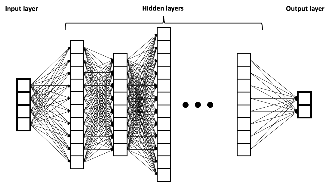
Fully-connected layers, also called feedforward or dense layers, refer to layers where each ‘node’ (a computing unit with a weight, bias and activation function) is connected to every node in the preceding and succeeding layers. It is often used in the final stages of a neural network to combine the features extracted by previous layers and produce the final output.

In our case we used fully-connected layers in the movement subnetwork to process the outputs of the convolutional layers into movement parameters than defined our movement kernel.
The Math
A fully connected layer in the neural network, maps an input vector \(\boldsymbol{u}\) of length \(n_u\) to an output vector \(\boldsymbol{o}\) of length \(n_o\) using \[ \mathbf{o} = \sigma(\mathbf{W} \mathbf{u} + \mathbf{b}), \]
where \(\sigma(\cdot)\) is referred to as the activation function and is applied element-wise to the argument. The matrix \(\mathbf{W}\) is an \(n_o \times n_u\) dense matrix of weights (with elements \(\mathbf{W}_{i,j} \in \mathbb{R}\)) that connects every element of the input vector to every element of the output vector, and \(\mathbf{b}\) is a vector of length \(n_o\) (with elements \(b_i \in \mathbb{R}\)) and is called the bias vector of the layer. Each fully connected layer in the neural network introduces \(n_o(n_u + 1)\) parameters that must be learned from the training data.
In our neural network architecture, the activation function is usually taken to be the rectified linear unit (ReLU) which is defined as \(\textup{ReLU}(x) = \max(x, 0)\). An exception to the use of ReLU in our model is where a fully-connected layer outputs a value that is taken to be the parameter of a density function. Our model has fully connected layers that predict the parameters of: (i) a two-component mixture of Von Mises densities; and (ii) a two-component mixture of Gamma densities. The former is used to model the direction for the next step in the animal’s trajectory and has parameters \(p_1\), \(p_2\), \(\kappa_1\), \(\kappa_2\), \(\mu_1\), and \(\mu_2\). The latter is used to model the step length of the next step in the trajectory and parameters relating to the mixture density, \(p_3\), \(p_4\), as well as shape parameters denoted \(\alpha_1\) and \(\alpha_2\) and scale parameters denoted \(\beta_1\) and \(\beta_2\) respectively. Each of these parameters have important bounds and we therefore use a different activation function to ensure that these bounds are honoured. For the parameters that can take any value in \((-\infty, \infty)\) (i.e. \(\mu_1\) and \(\mu_2\)), the activation function used is simply the identity function: \(\sigma(x) = x\). For the parameters that are required to be greater than zero (i.e. \(\alpha\), \(\beta\), \(\kappa_1\), and \(\kappa_2\)), the activation function used is the exponential function: \(\sigma(x) = \exp(x)\). For the mixture proportions, \(p_1 + p_2\) and \(p_3 + p_4\) must each sum to exactly 1, so we normalised them via \(p_1 = p_1/(p_1 + p_2)\), \(p_2 = p_2/(p_1 + p_2)\) and \(p_3 = p_3/(p_3 + p_4)\), \(p_4 = p_4/(p_3 + p_4)\). As one \(p\) can be identified from the other, we could have also used a single \(p\) for each mixture density, and normalised it using the logistic activation function \(\sigma(x) = 1/(1 + \exp(-x))\) to be in the interval \([0, 1]\), and then used \(1-p\) for the remaining mixture proportion.
Max Pooling
Max pooling is an operation that is often used in convolutional neural networks to reduce dimensionality and condense information. Here we present a typical way that max pooling is applied in practice (and how it is applied in our model). The max pooling operation is best thought of as a function that accepts an \(a \times a\) matrix, \(\mathbf{A}\), as input and outputs an \(a^{\star} \times a^{\star}\) matrix \(\mathbf{A}^{\star}\), where \(a^{\star} = \frac{a}{k}\). For simplicity here, we assume that \(\frac{a}{k}\) is integer-valued, but where this is not the case, the dimensions of the matrix \(\mathbf{A}\) can be modified using “padding” to augment the matrix with additional rows and columns at it’s edges.
We refer to \(k\) as the kernel-width in the max pooling operation and use this to partition the matrix \(\mathbf{A}\) as
\[\mathbf{A} = \left(\begin{array}{cccc} \mathbf{A}_{1, 1} & \mathbf{A}_{1, 2} & \dots & \mathbf{A}_{1, a^{\star}} \\ \mathbf{A}_{2, 1} & \mathbf{A}_{2, 2} & \dots & \mathbf{A}_{2, a^{\star}} \\ \vdots & \vdots & \ddots & \vdots \\ \mathbf{A}_{a^{\star}, 1} & \mathbf{A}_{a^{\star}, 2} & \dots & \mathbf{A}_{a^{\star}, a^{\star}} \end{array}\right),\]
where each sub-matrix \(\mathbf{A}_{i, j}\) \((i, j \in \{1, \dots, a^{\star} \})\) is of dimension \(k \times k\). The output of the max pooling operation is the matrix \(\mathbf{A}^{\star}\) which we define as
\[\mathbf{A}^{\star} = \left(\begin{array}{cccc} \max(\mathbf{A}_{1, 1}) & \max(\mathbf{A}_{1, 2}) & \dots & \max(\mathbf{A}_{1, a^{\star}}) \\ \max(\mathbf{A}_{2, 1}) & \max(\mathbf{A}_{2, 2}) & \dots & \max(\mathbf{A}_{2, a^{\star}}) \\ \vdots & \vdots & \ddots & \vdots \\ \max(\mathbf{A}_{a^{\star}, 1}) & \max(\mathbf{A}_{a^{\star}, 2}) & \dots & \max(\mathbf{A}_{a^{\star}, a^{\star}}) \end{array}\right).\]
Max pooling can therefore be seen as simultaneously reducing the dimension of a matrix by a factor of \(k\), and highlighting the extremes of the input feature matrix \(\mathbf{A}\) over space.
In practice, max pooling operations often follow two-dimensional convolutional blocks in a neural network model. Where the convolutional blocks have more than one filter, the input to the max pooling operation will actually be an \(a \times a \times F\) tensor (a three-dimensional array), where \(F\) is the number of filters that are learned by the model in each convolutional layer. In this case, the max pooling operation described above is simply applied independently to each of \(F\) matrices of size \(a \times a\) and each of the \(a^{\star} \times a^{\star}\) sub-matrices are stacked to create a \(a^{\star} \times a^{\star} \times f\) tensor that is passed to the next layer in the network (often another convolutional layer).