deepSSF Data Prep
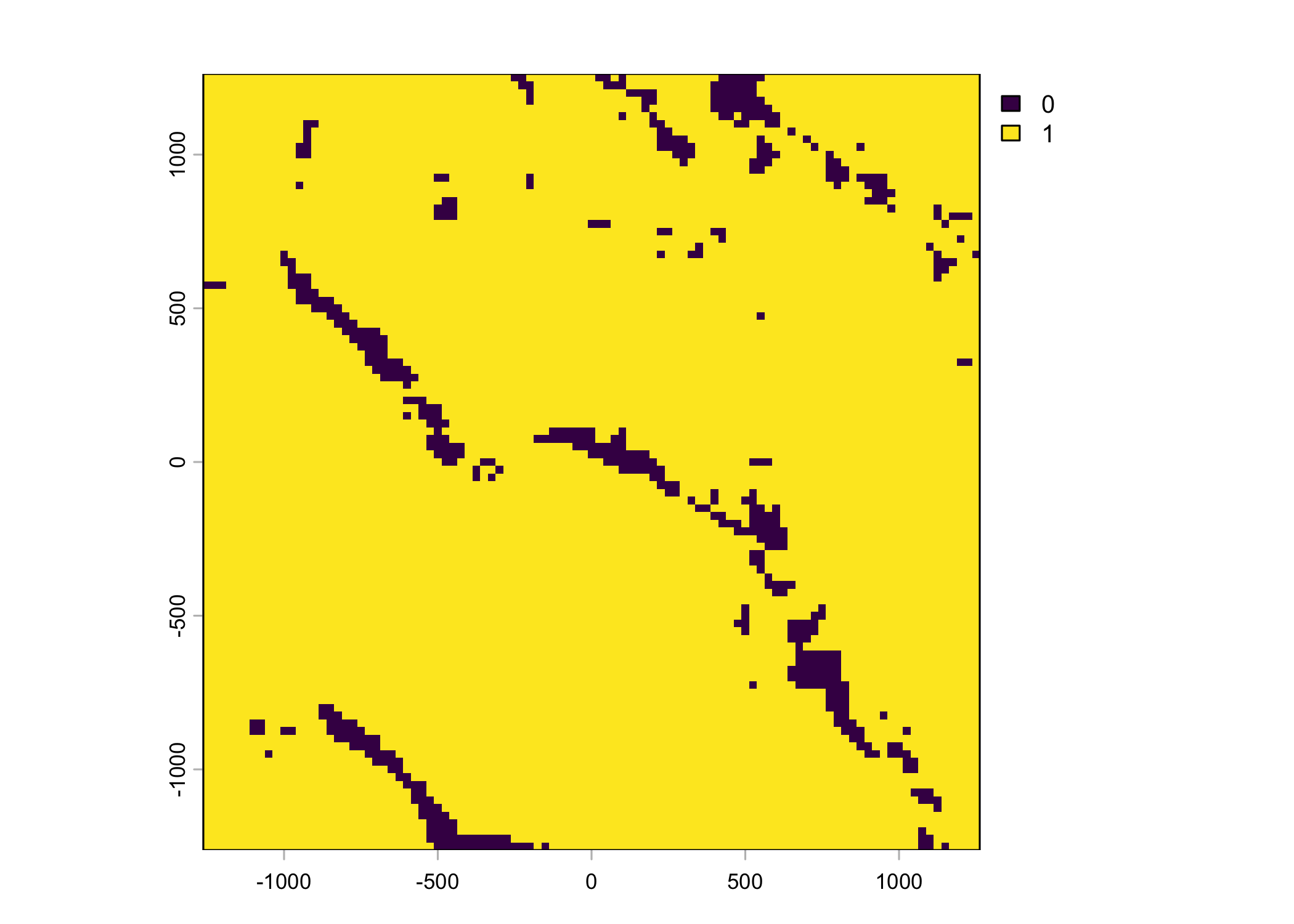
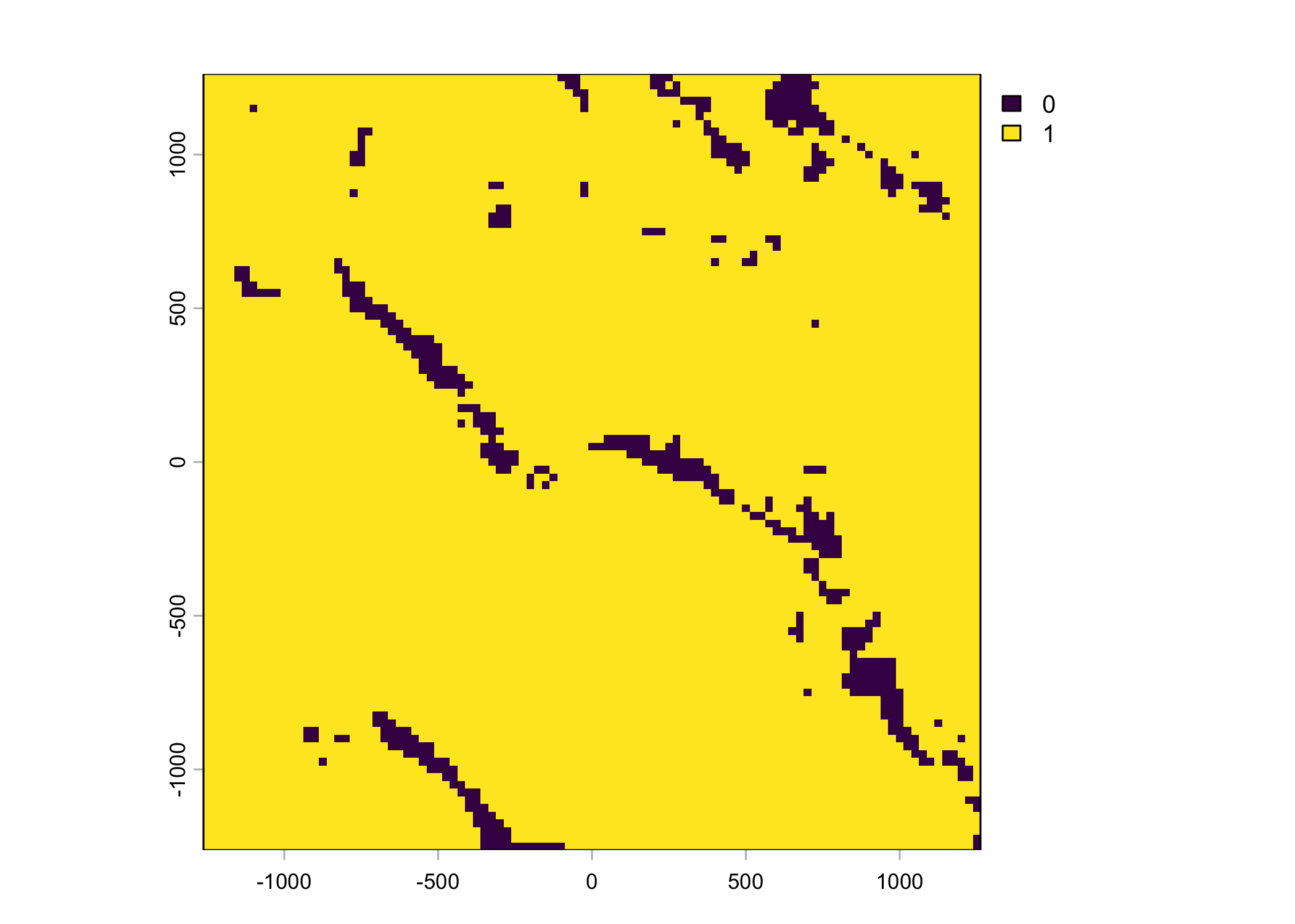
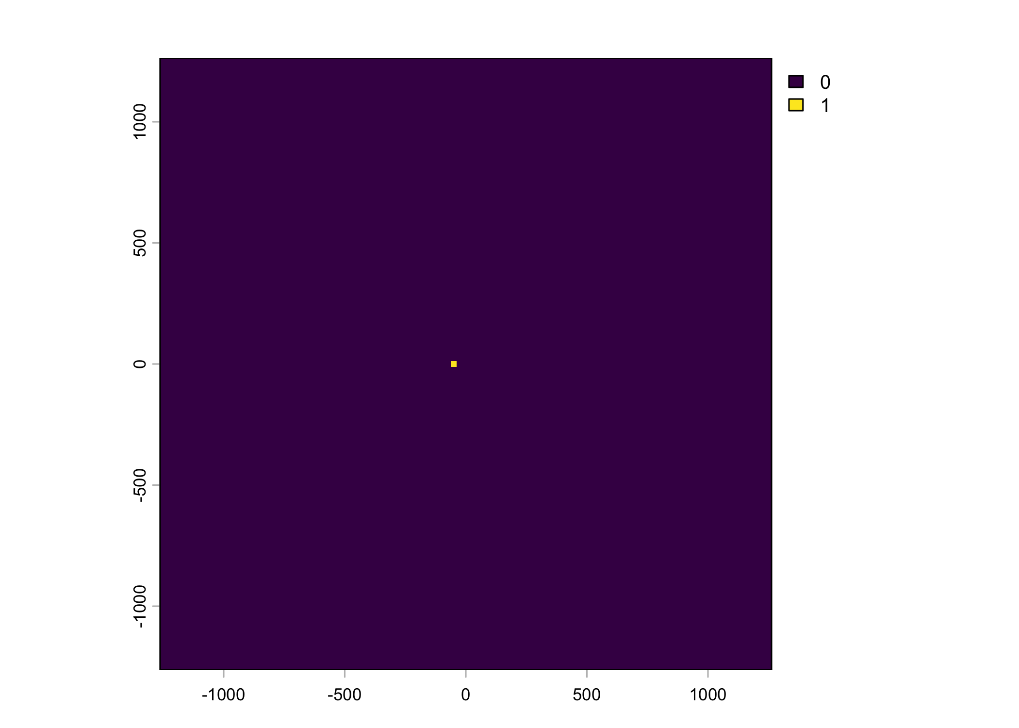
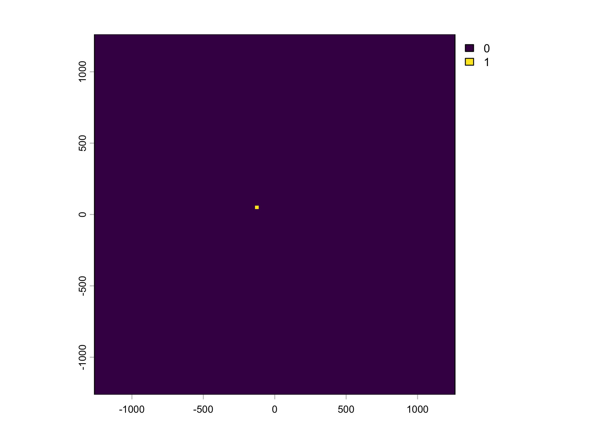
Here we prepare the data for fitting a deepSSF model. We load the GPS data and tidy it, create a trajectory object containing a series of steps and read in the environmental layers. For each observed step we crop out local subsets of the environmental layers, centred on the step’s location. For every step we will then have the surrounding environmental information stored as a stack of small rasters, with the ‘target’ of what we’re trying to predict (the actual location of the next step) as a raster layer as well, with all cells being 0 except the observed next location, which is 1. These, along with temporal covariates and the previous bearing, will be the input data for the deepSSF model.
Loading packages
Import data
New names:
Rows: 133161 Columns: 11
── Column specification
──────────────────────────────────────────────────────── Delimiter: "," chr
(3): node, dates, DateTime dbl (7): ...1, lat, lon, height, accuracy, heading,
speed dttm (1): timestamp
ℹ Use `spec()` to retrieve the full column specification for this data. ℹ
Specify the column types or set `show_col_types = FALSE` to quiet this message.
• `` -> `...1`Tidy data
Code
# remove individuals that have poor data quality or less than about 3 months of data.
# The "2014.GPS_COMPACT copy.csv" string is a duplicate of ID 2024, so we also exclude it
buffalo <- buffalo %>% filter(!node %in% c("2014.GPS_COMPACT copy.csv",
# 2005, 2014, 2018, 2021, 2022, 2024,
2029, 2043, 2265, 2284, 2346, 2354))
# arrange by time and exclude any duplicate timestamps (within the same individual's data)
buffalo <- buffalo %>%
group_by(node) %>%
arrange(DateTime, .by_group = T) %>%
distinct(DateTime, .keep_all = T) %>%
arrange(node) %>%
mutate(ID = node)
# keep only the relevant columns
buffalo_clean <- buffalo[, c(12, 2, 4, 3)]
# rename the columns
colnames(buffalo_clean) <- c("id", "time", "lon", "lat")
# convert the time to the correct timezone
attr(buffalo_clean$time, "tzone") <- "Australia/Queensland"
head(buffalo_clean)[1] "Australia/Queensland"Create a subset of the data to export for testing the deepSSF package
We’ll select the ID 2005, as that was used for training the model in the MEE paper
Code
buffalo_clean_2005 <- buffalo_clean %>% filter(id == 2005)
# convert to sf object and transform to the same projection as the covariates (GDA94 / Geoscience Australia Lambert, EPSG:3112)
buffalo_clean_2005_sf <- buffalo_clean_2005 %>%
st_as_sf(coords = c("lon", "lat"), crs = 4326) %>%
st_transform(crs = 3112)
# add the coordinates back to the data frame
buffalo_clean_2005_coords <- buffalo_clean_2005_sf %>%
st_coordinates() %>%
as.data.frame() %>%
rename(x = X, y = Y)
buffalo_clean_2005_proj <- buffalo_clean_2005 %>%
bind_cols(buffalo_clean_2005_coords) %>%
dplyr::select(id, time, x, y)
buffalo_clean_2005_proj %>% write_csv("data/buffalo_djelk_id2005.csv")Setup trajectory
Use the amt package to create a trajectory object from the cleaned data.
Code
buffalo_all <- buffalo_clean %>% mk_track(id = id,
lon,
lat,
time,
all_cols = T,
crs = 4326) %>%
# Transformation to GDA94 / Geoscience Australia Lambert (https://epsg.io/3112)
transform_coords(crs_to = 3112, crs_from = 4326) %>% arrange(id)
# Number of IDs and locations
buffalo_all %>%
summarise(n_ids = n_distinct(id),
n_locations = n())Plot the data coloured by time
Code
Plot a timeline of each individual
Code
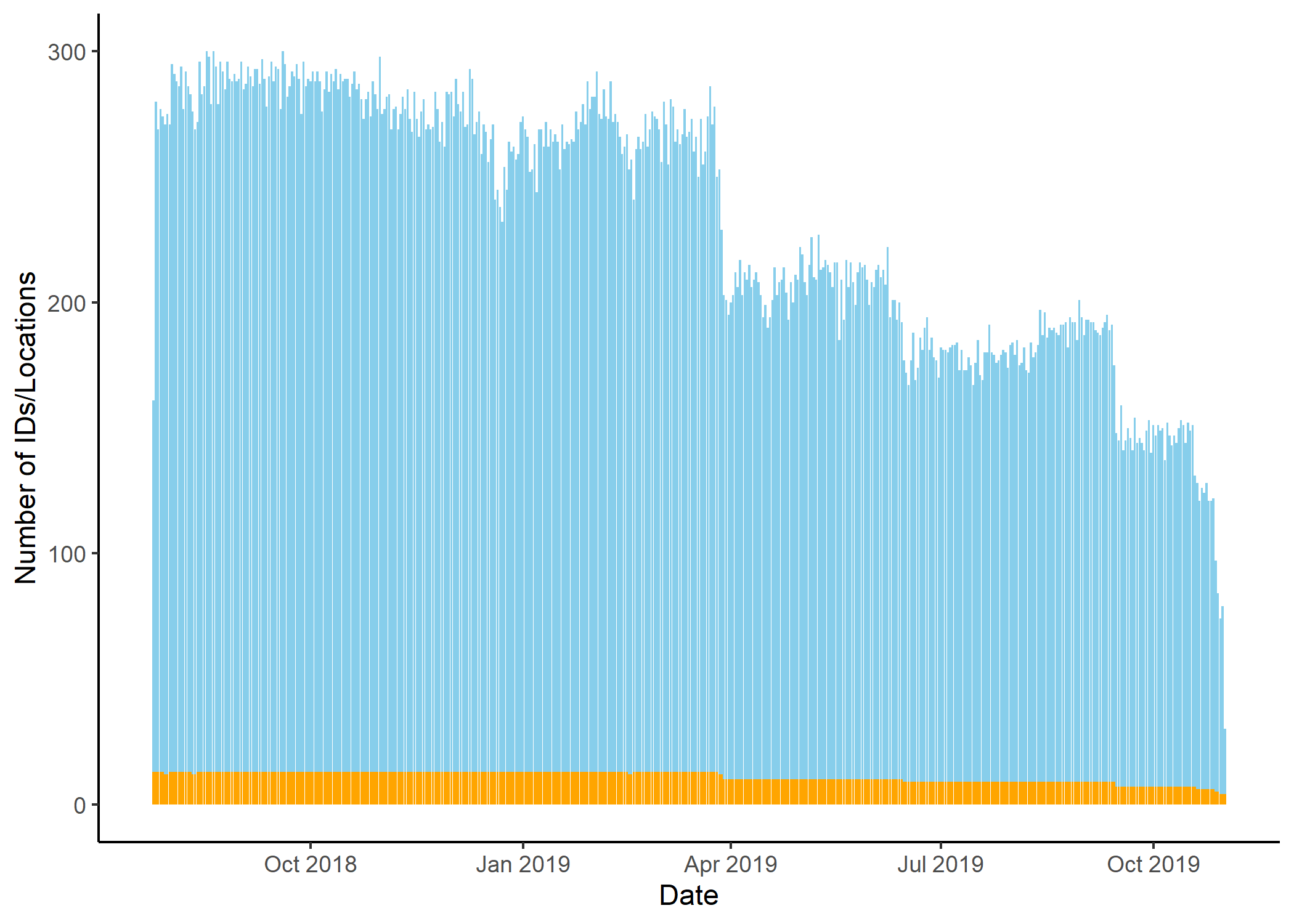
Number of location per day
Code
buffalo_daily_locations <- buffalo_all %>%
mutate(date = lubridate::date(t_)) %>%
dplyr::group_by(date) %>%
summarise(
n_locations = n(),
n_individuals = n_distinct(id)
)
buffalo_daily_locations %>%
ggplot() +
geom_col(aes(x = date, y = n_locations),
fill = "skyblue") +
geom_col(aes(x = date, y = n_individuals),
fill = "orange") +
scale_x_date("Date") +
scale_y_continuous("Number of IDs/Locations") +
scale_colour_viridis_d() +
theme_classic() +
theme(legend.position = "none") 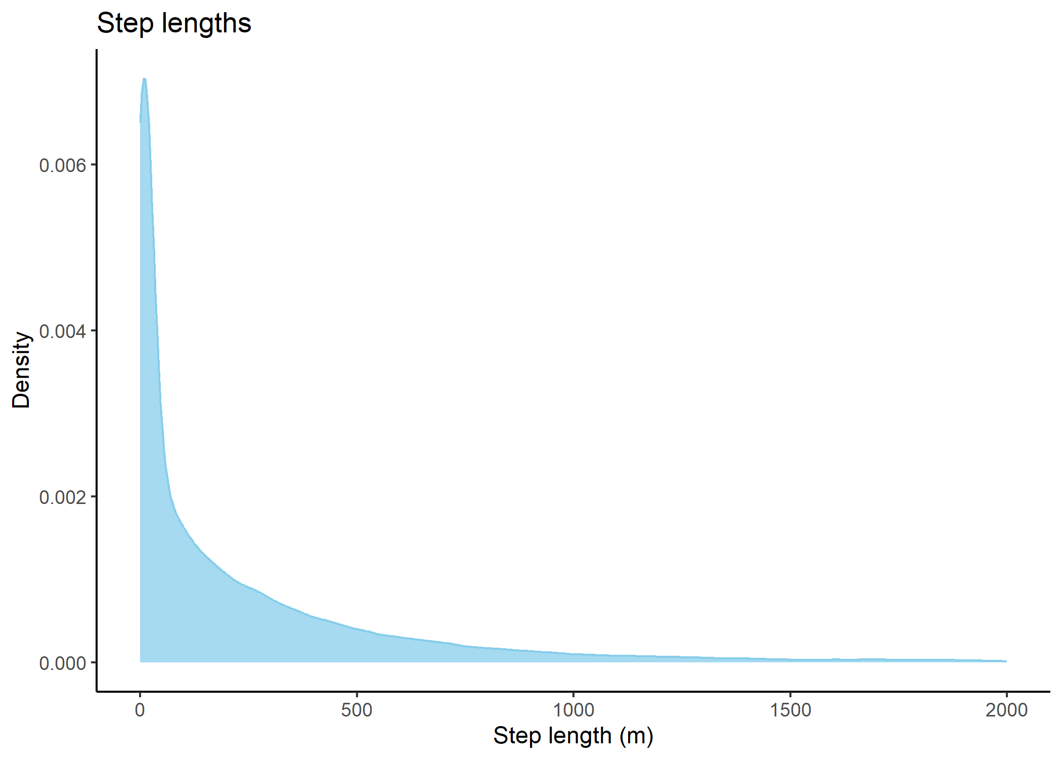
Generating the data to fit a deepSSF model
Create a steps object to check the step lengths
Code
# nest the data by individual
buffalo_all_nested <- buffalo_all %>% arrange(id) %>% nest(data = -"id")
buffalo_all_nested_steps <- buffalo_all_nested %>%
mutate(steps = map(data, function(x)
x %>%
# track_resample(rate = hours(1), tolerance = minutes(10)) %>%
steps()))
# unnest the data after creating 'steps' objects
buffalo_all_steps <- buffalo_all_nested_steps %>%
amt::select(id, steps) %>%
amt::unnest(cols = steps)
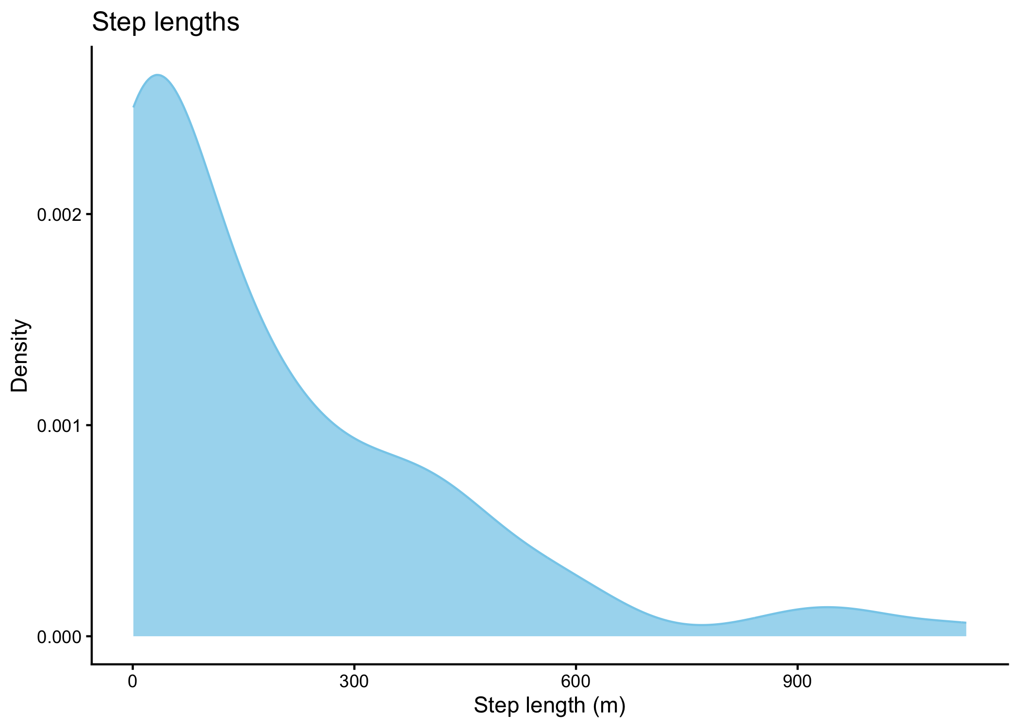
head(buffalo_all_steps)Plot step lengths and set the buffer distance
Code
# plot step lengths
buffalo_all_steps %>%
filter(sl_ < 2000) %>%
ggplot() +
geom_density(aes(x = sl_), #, bins = 50
fill = "skyblue", colour = "skyblue", alpha = 0.75) +
# scale_x_continuous("Step length (m)") + #, limits = c(-25, 1250)
scale_x_log10("Step length (m)") + #, limits = c(-25, 1250)
scale_y_continuous("Density") +
ggtitle("Step lengths") +
theme_classic()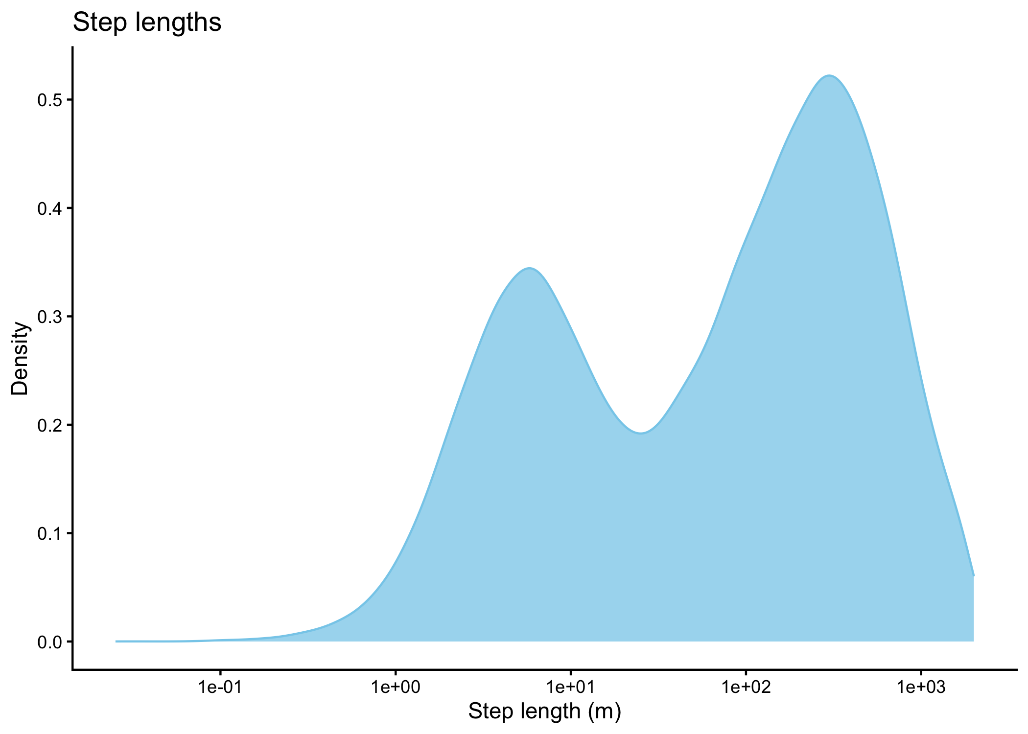
Code
[1] TRUECode
[1] "Number of cells in each axis: 101"Code
[1] "Proportion of steps less than 1262.5m in x or y direction: 0.9637"Code
[1] "Maximum distance at corner: 1785.44"Prepare and export data for single layer saving (Python script)
We also have another script that saves all local layers as individual npy arrays, which works better when there are many steps per id (to prevent large tif files), and can make things a bit easier for training models with many ids.
Code
buffalo_all_steps_save <- buffalo_all_steps %>% mutate(
dt_minute = as.numeric(round(difftime(t2_, t1_, units = "mins"), 0)),
dt_hour = as.numeric(round(difftime(t2_, t1_, units = "hours"), 2)),
# add the minutes as a decimal to the hour, and the hour as a decimal to the day
hour_t1 = round(lubridate::hour(t1_) + lubridate::minute(t1_)/60,2),
yday_t1 = round(lubridate::yday(t1_) + lubridate::hour(t1_)/24,2),
hour_t1_sin1 = sin(2*pi*hour_t1/24),
hour_t1_cos1 = cos(2*pi*hour_t1/24),
hour_t1_sin2 = sin(4*pi*hour_t1/24),
hour_t1_cos2 = cos(4*pi*hour_t1/24),
yday_t1_sin1 = sin(2*pi*yday_t1/365.25),
yday_t1_cos1 = cos(2*pi*yday_t1/365.25),
yday_t1_sin2 = sin(4*pi*yday_t1/365.25),
yday_t1_cos2 = cos(4*pi*yday_t1/365.25),
# add the minutes as a decimal to the hour, and the hour as a decimal to the day
hour_t2 = round(lubridate::hour(t2_) + lubridate::minute(t2_)/60,2),
yday_t2 = round(lubridate::yday(t2_) + lubridate::hour(t2_)/24,2),
bearing = direction_p,
bearing_sin = sin(bearing),
bearing_cos = cos(bearing)
)
buffalo_all_steps_saveSave the data to a csv file
Code
In our case over 96% of the steps were less than a distance of 1262.5m in either the x or y direction, which would mean that including 101 x 101 cells (which would be 2525 m x 2525 m) would include at least 96% of the steps. As the distance is further to the corner (but still less than the buffer distance in the x and y directions), there will be step lengths longer than the buffer distance (up to 1785 m).
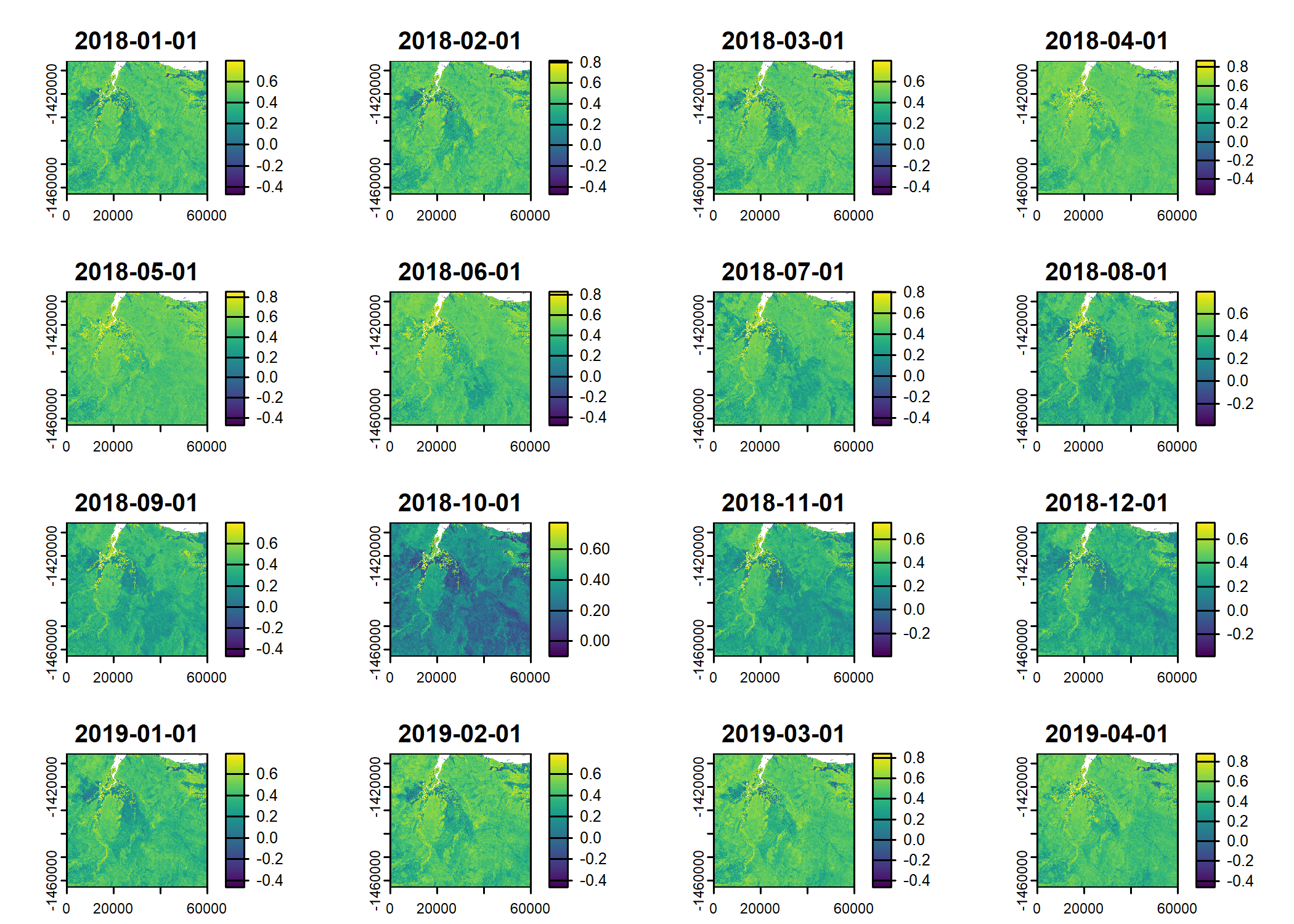
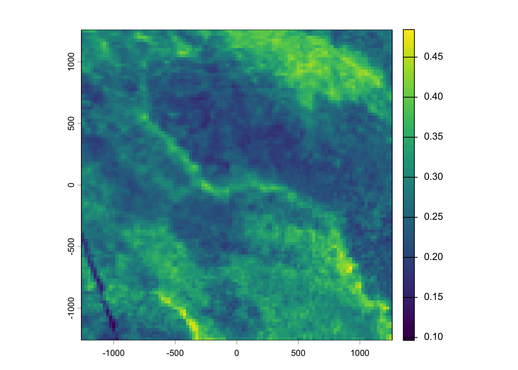
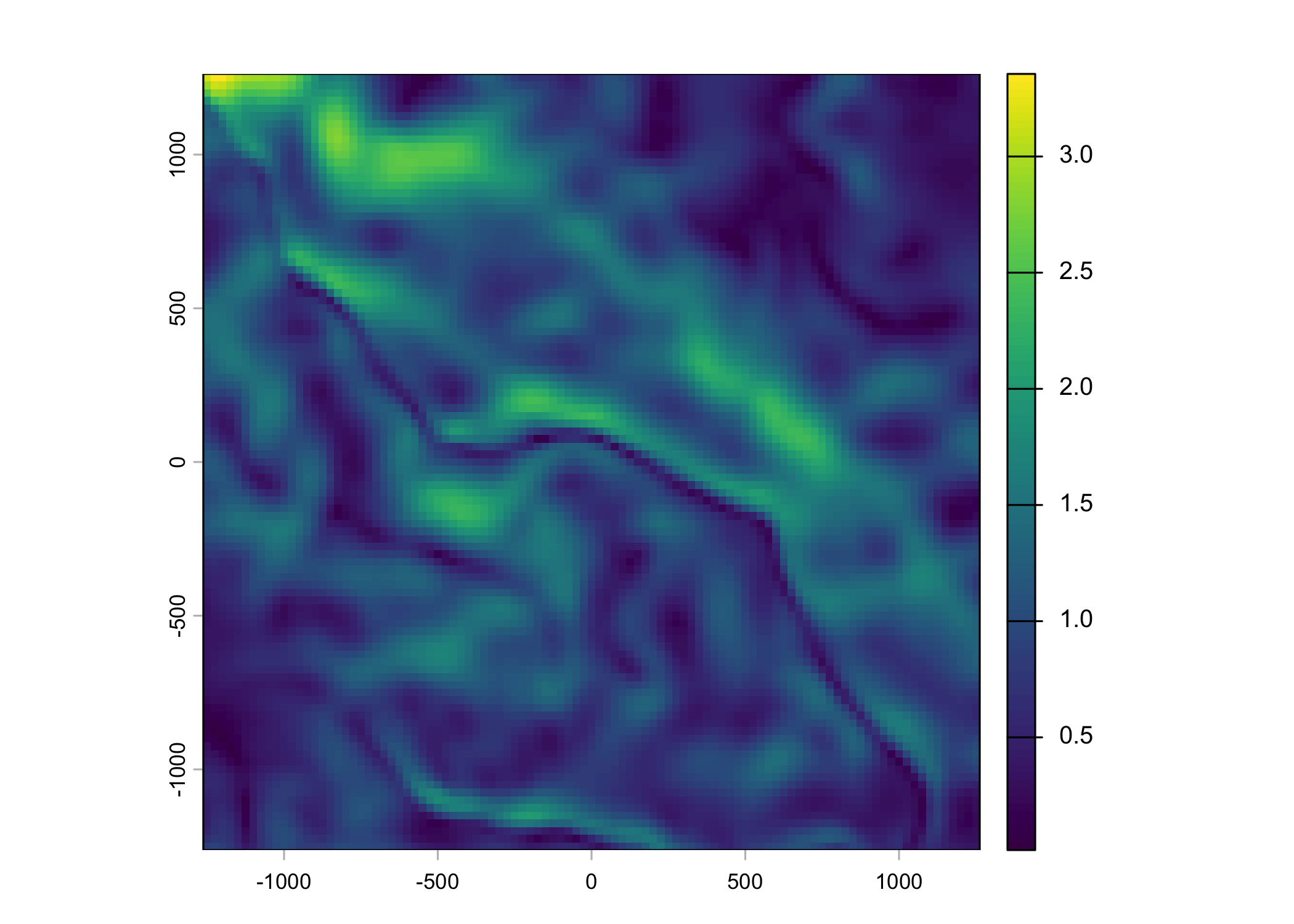
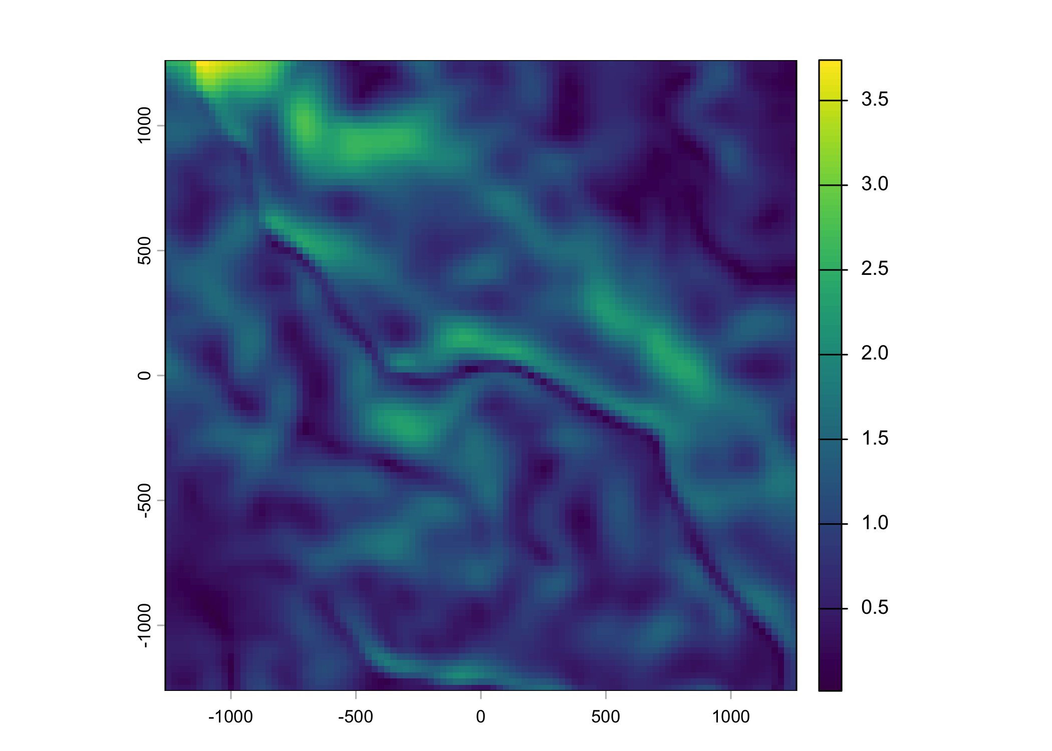
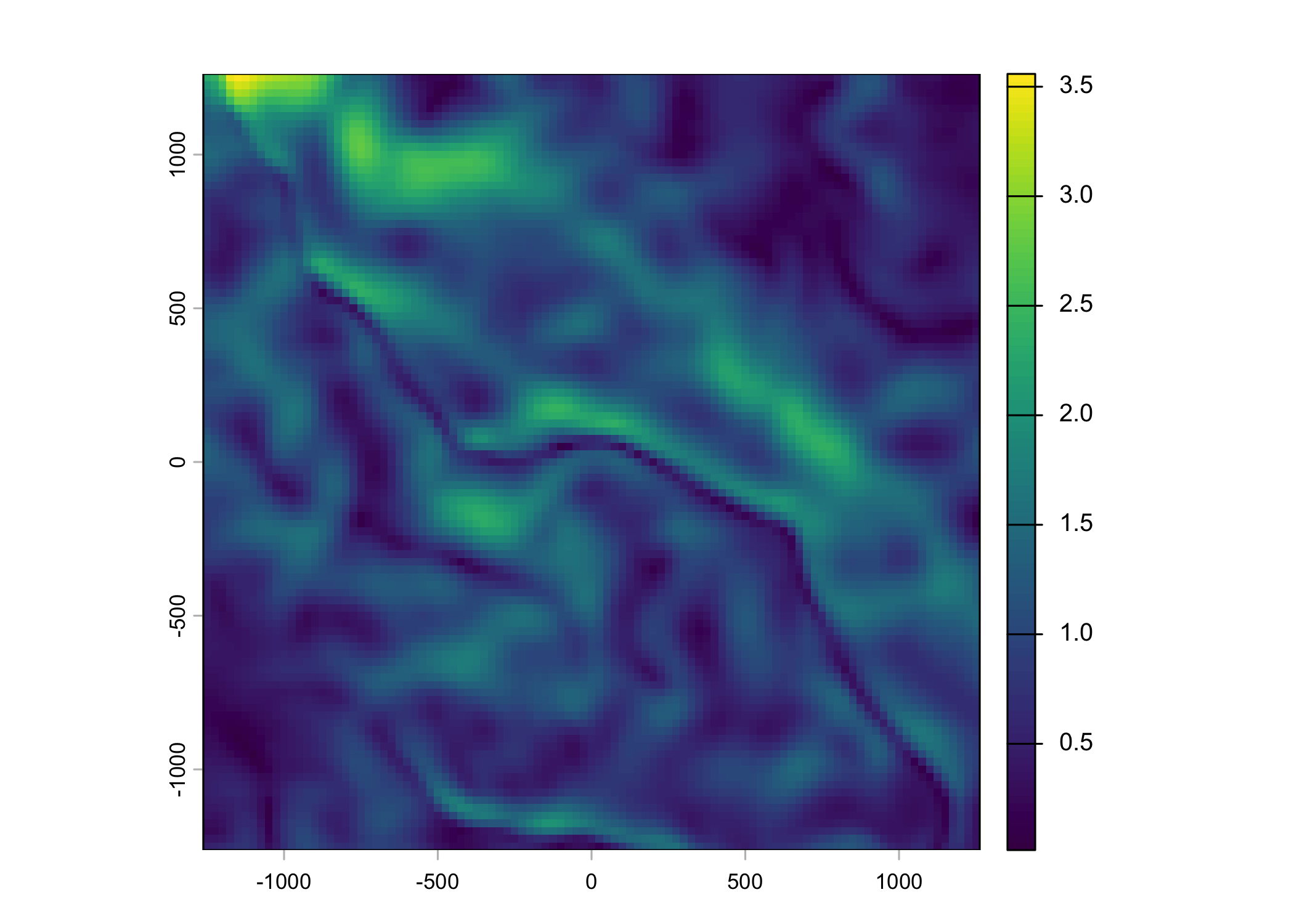
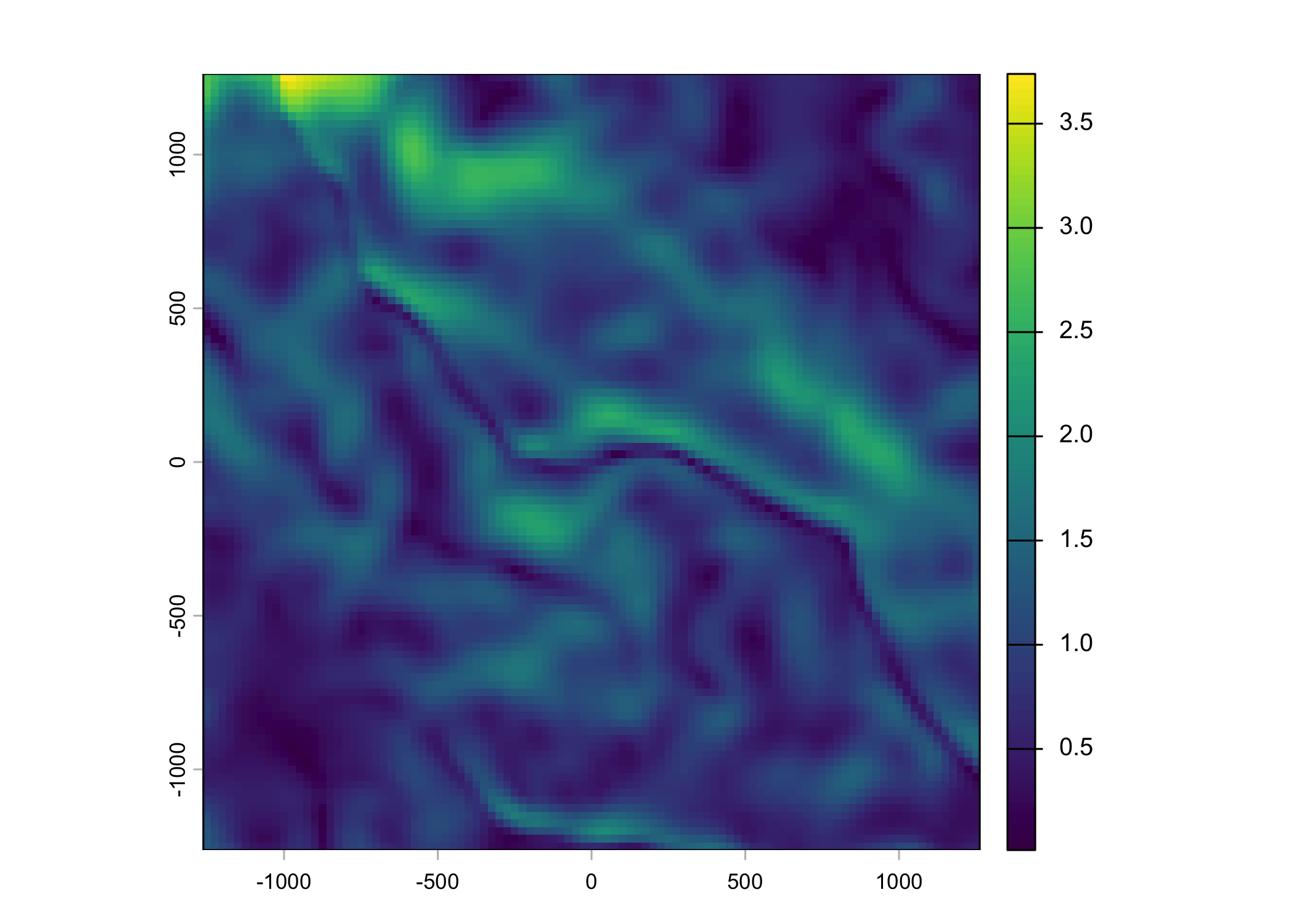
Read in the environmental covariates
Code
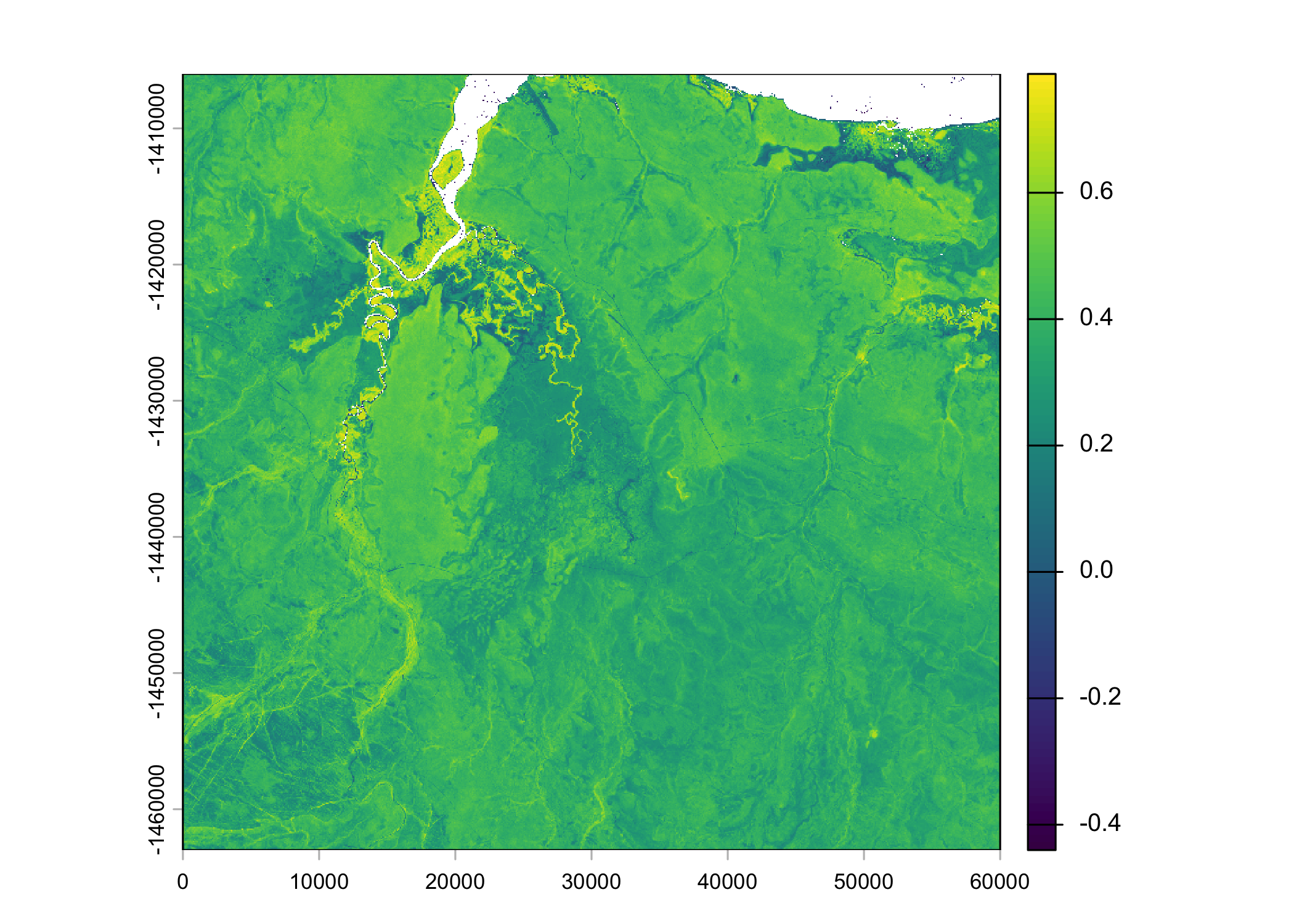
ndvi_projected <- rast("mapping/cropped rasters/ndvi_GEE_projected_watermask20230207.tif")
terra::time(ndvi_projected) <- as.POSIXct(lubridate::ymd("2018-01-15") + months(0:23))
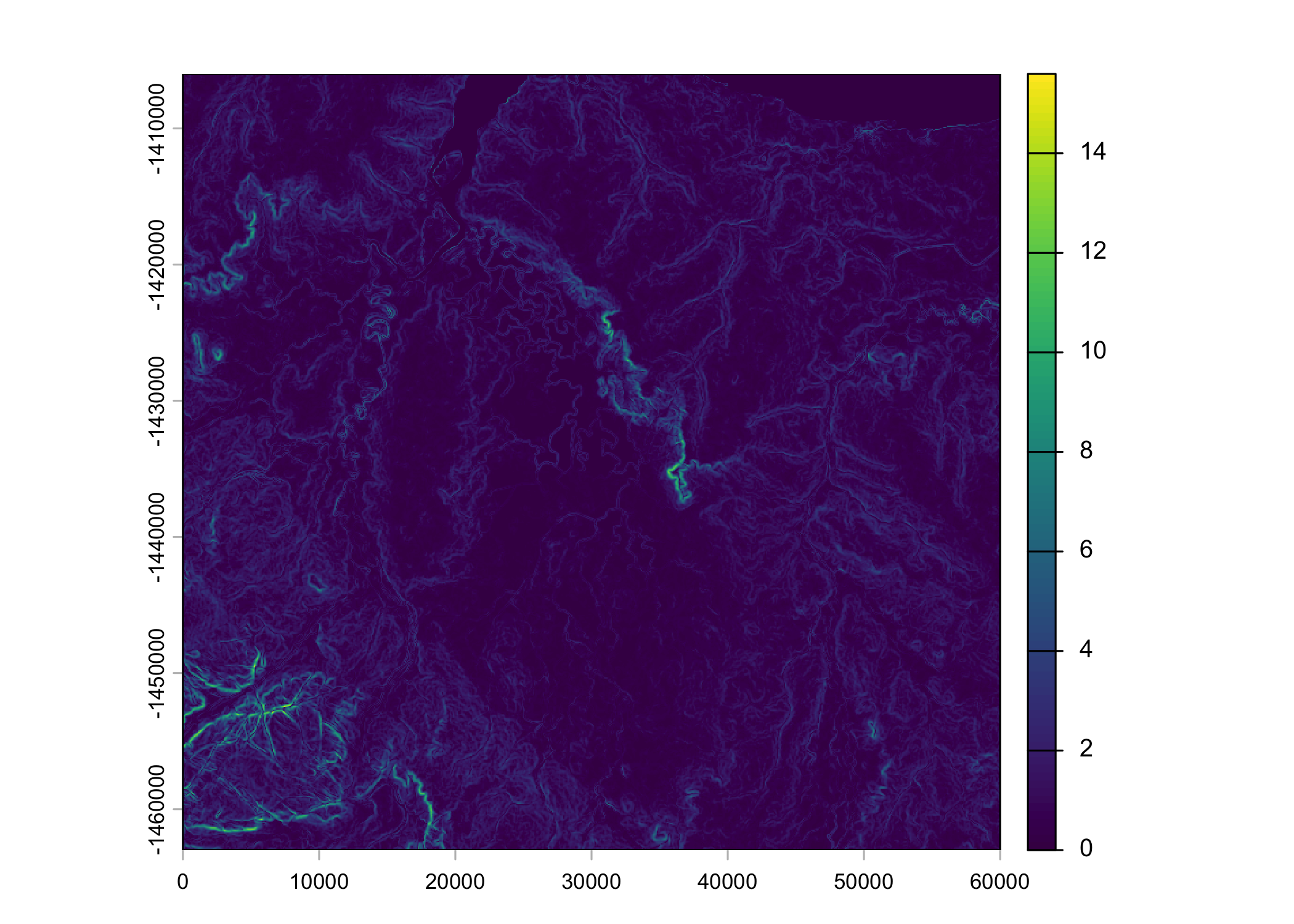
slope <- rast("mapping/cropped rasters/slope_raster.tif")
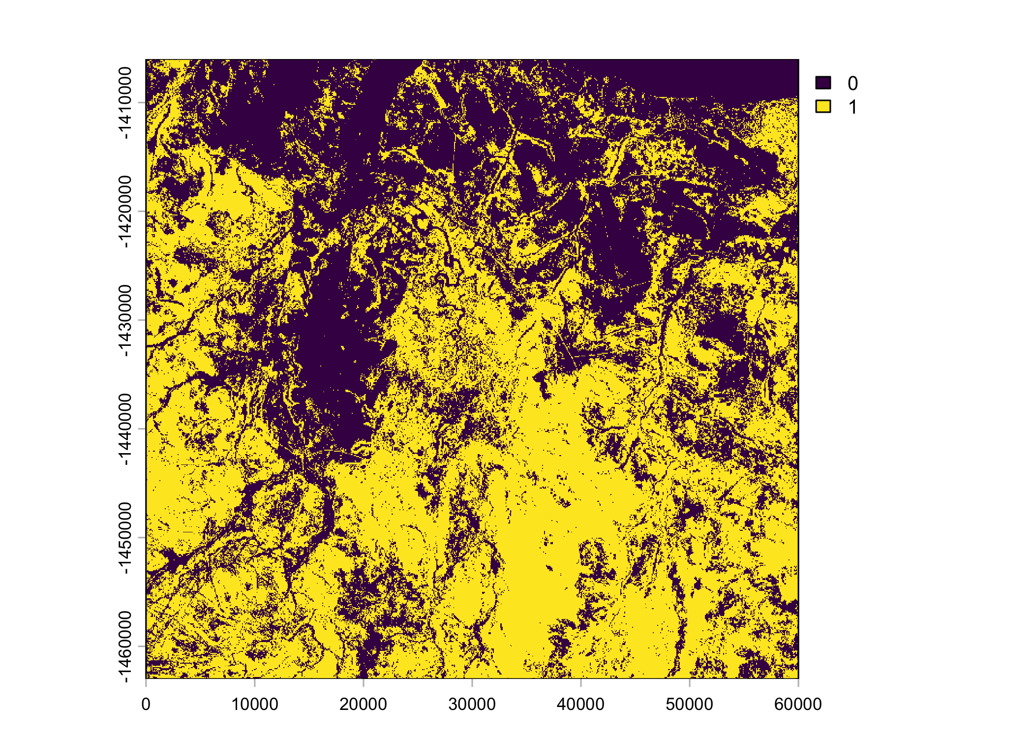
veg_herby <- rast("mapping/cropped rasters/veg_herby.tif")
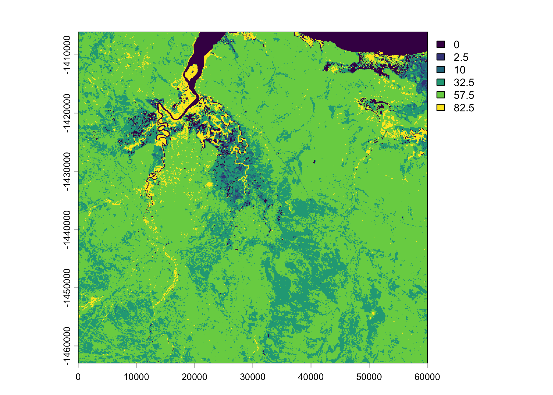
canopy_cover <- rast("mapping/cropped rasters/canopy_cover.tif")
# change the names (these will become the column names when extracting
# covariate values at the used and random steps)
names(ndvi_projected) <- rep("ndvi", terra::nlyr(ndvi_projected))
names(slope) <- "slope"
names(veg_herby) <- "veg_herby"
names(canopy_cover) <- "canopy_cover"
# to plot the rasters
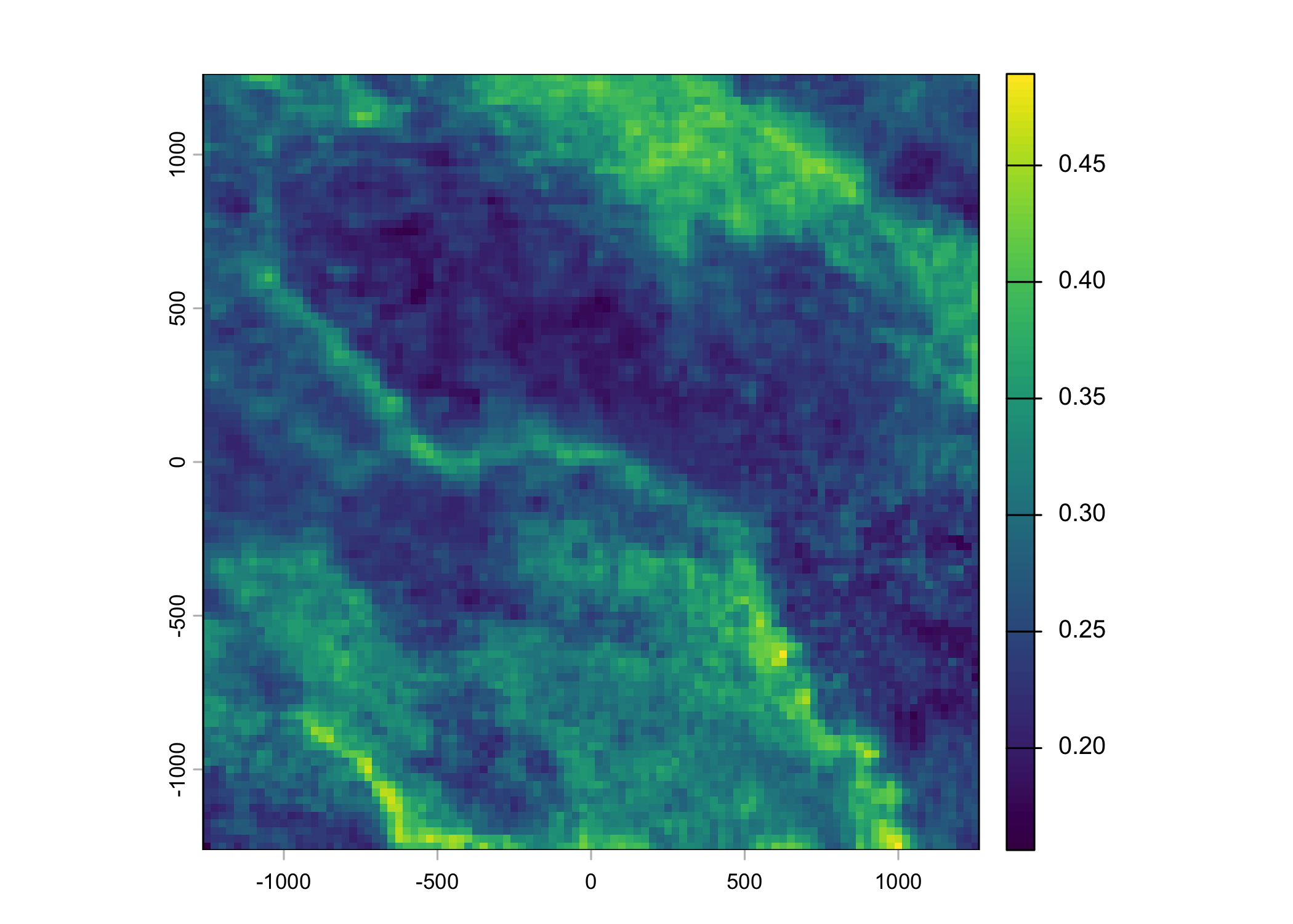
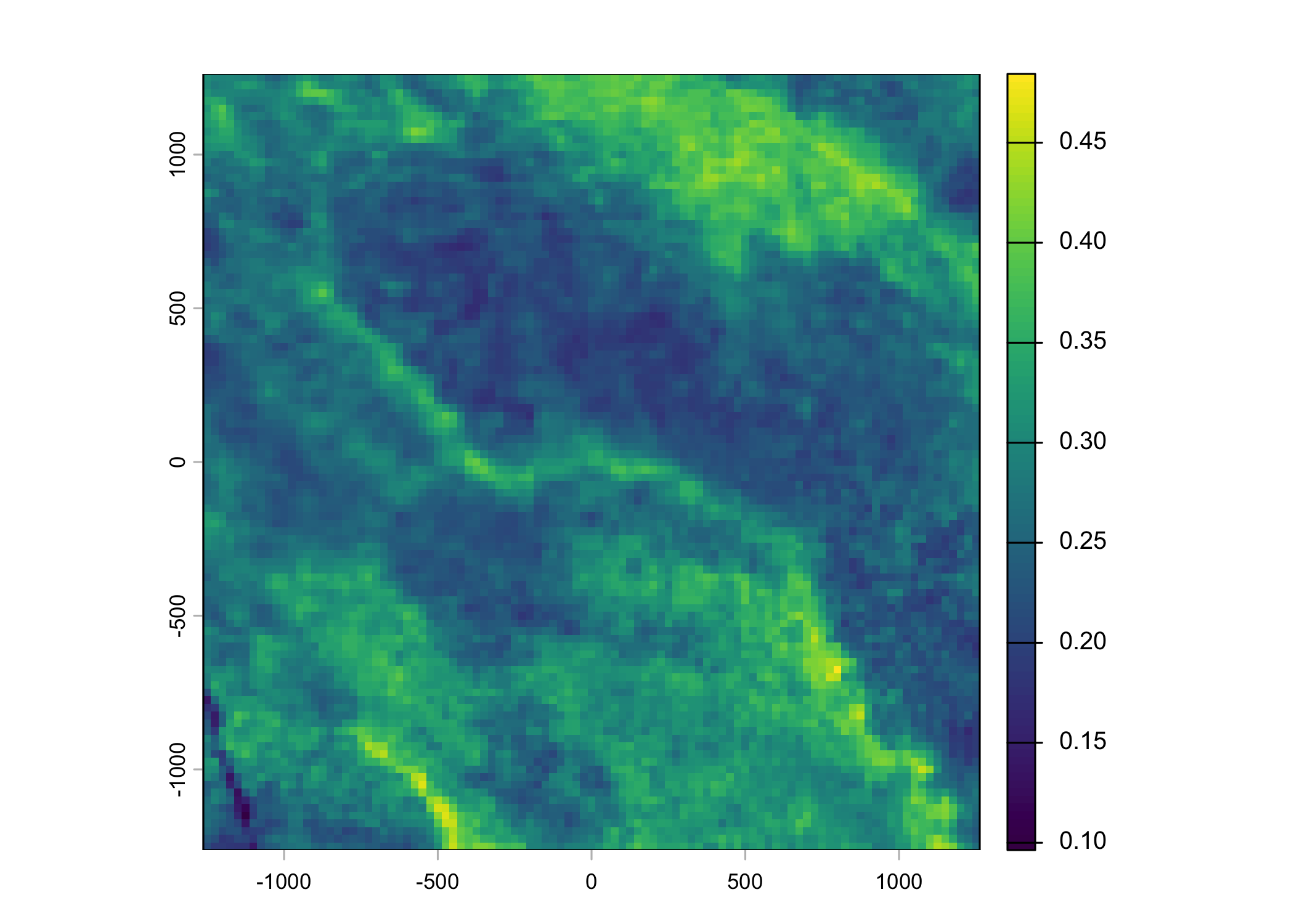
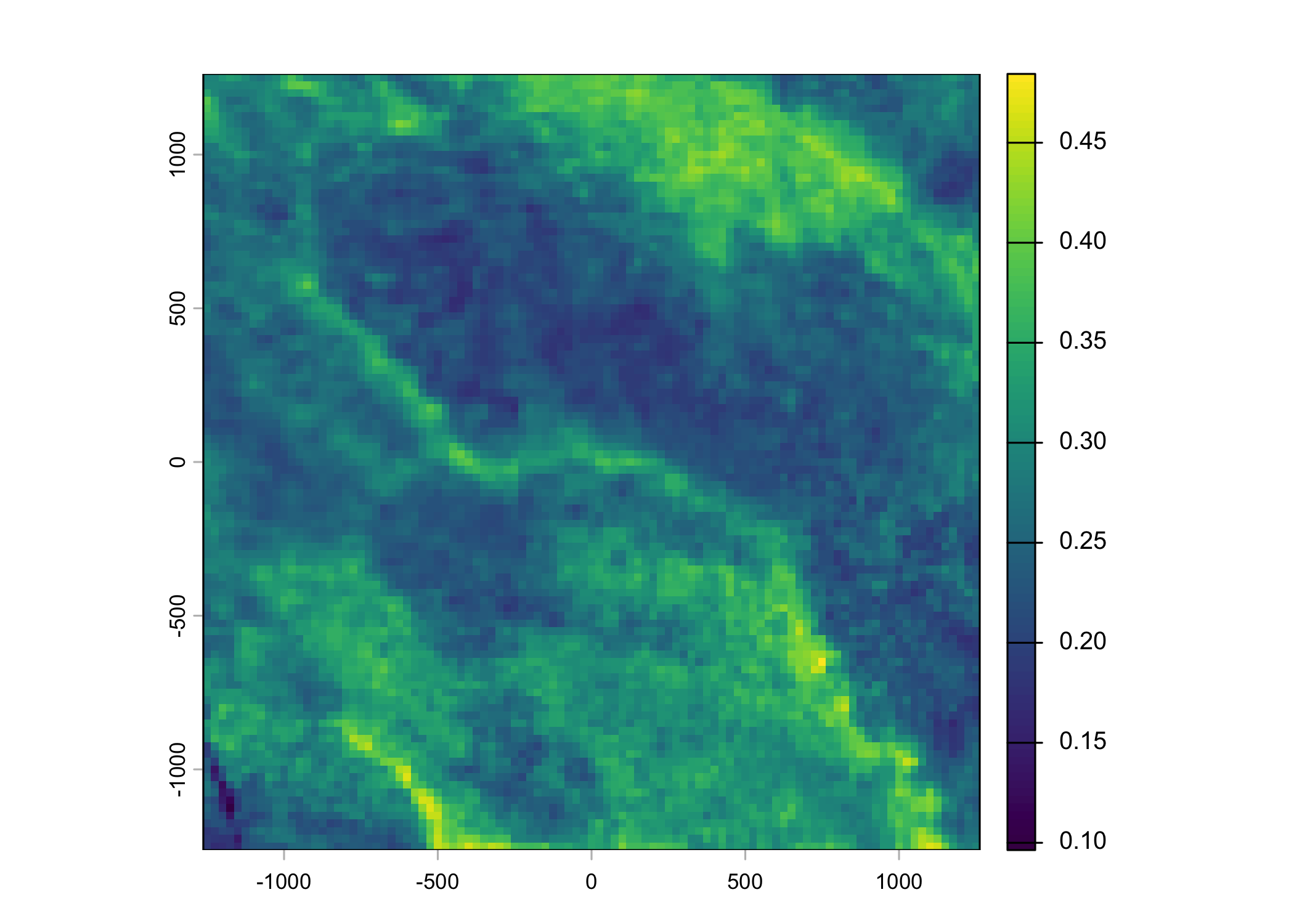
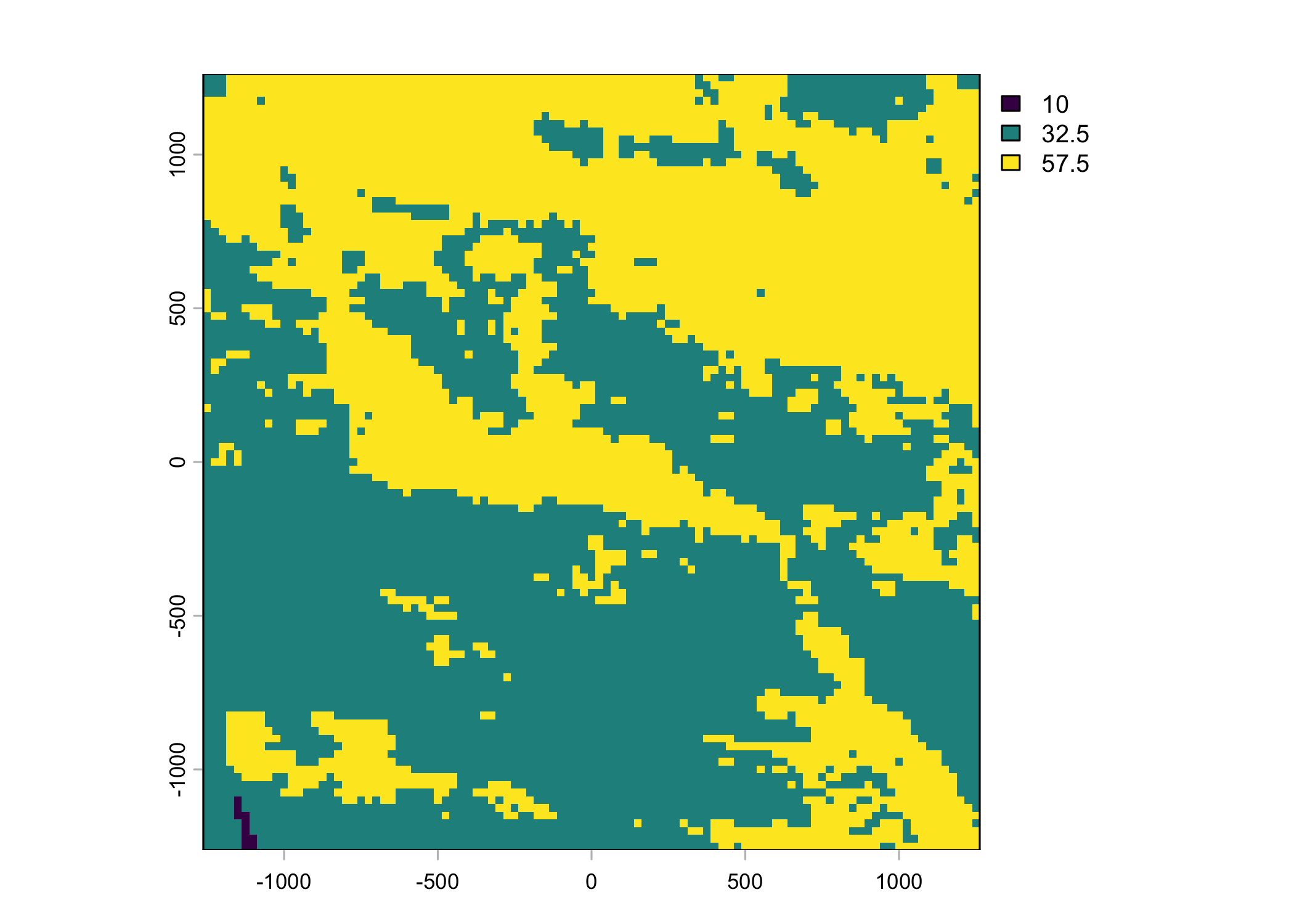
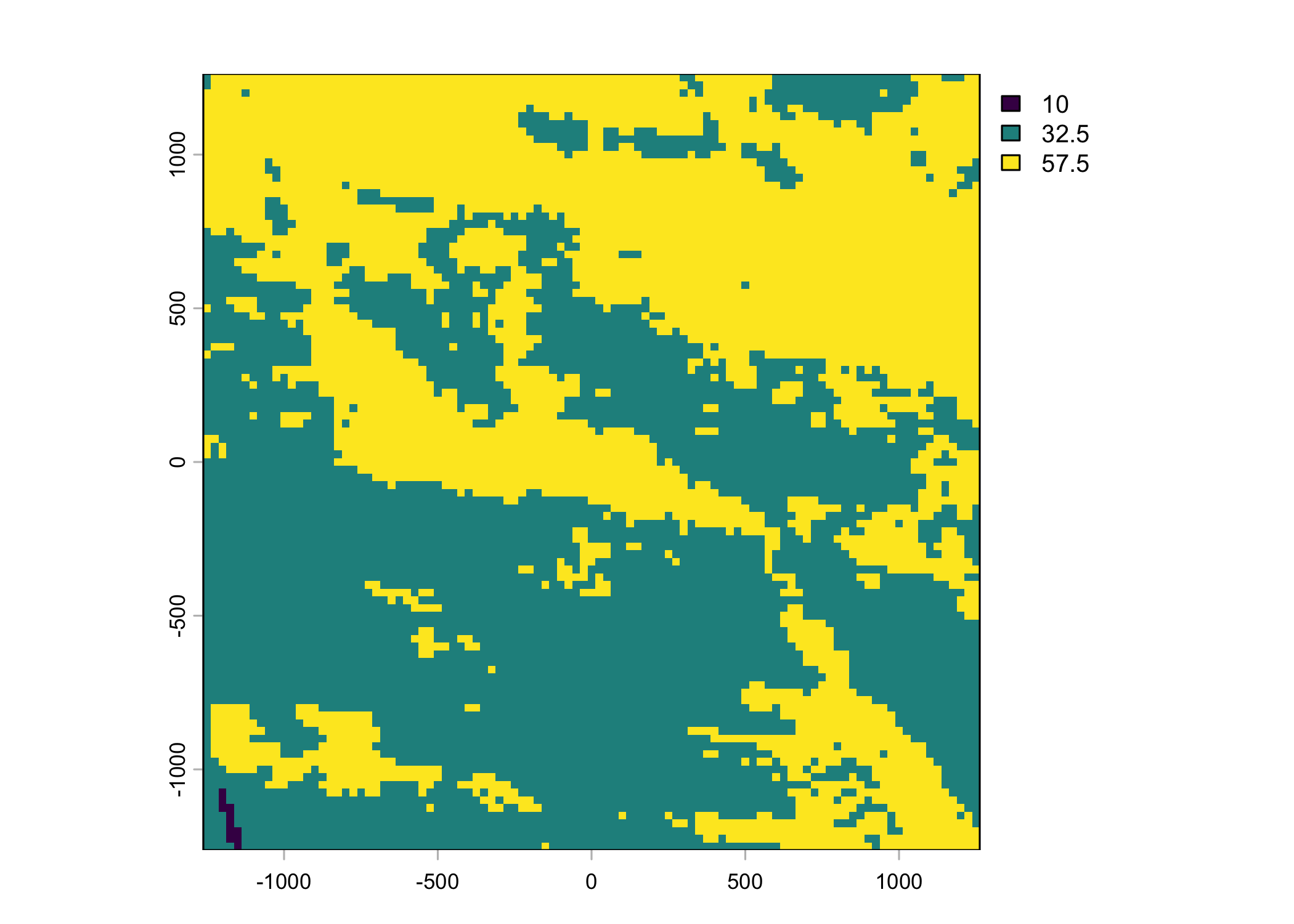
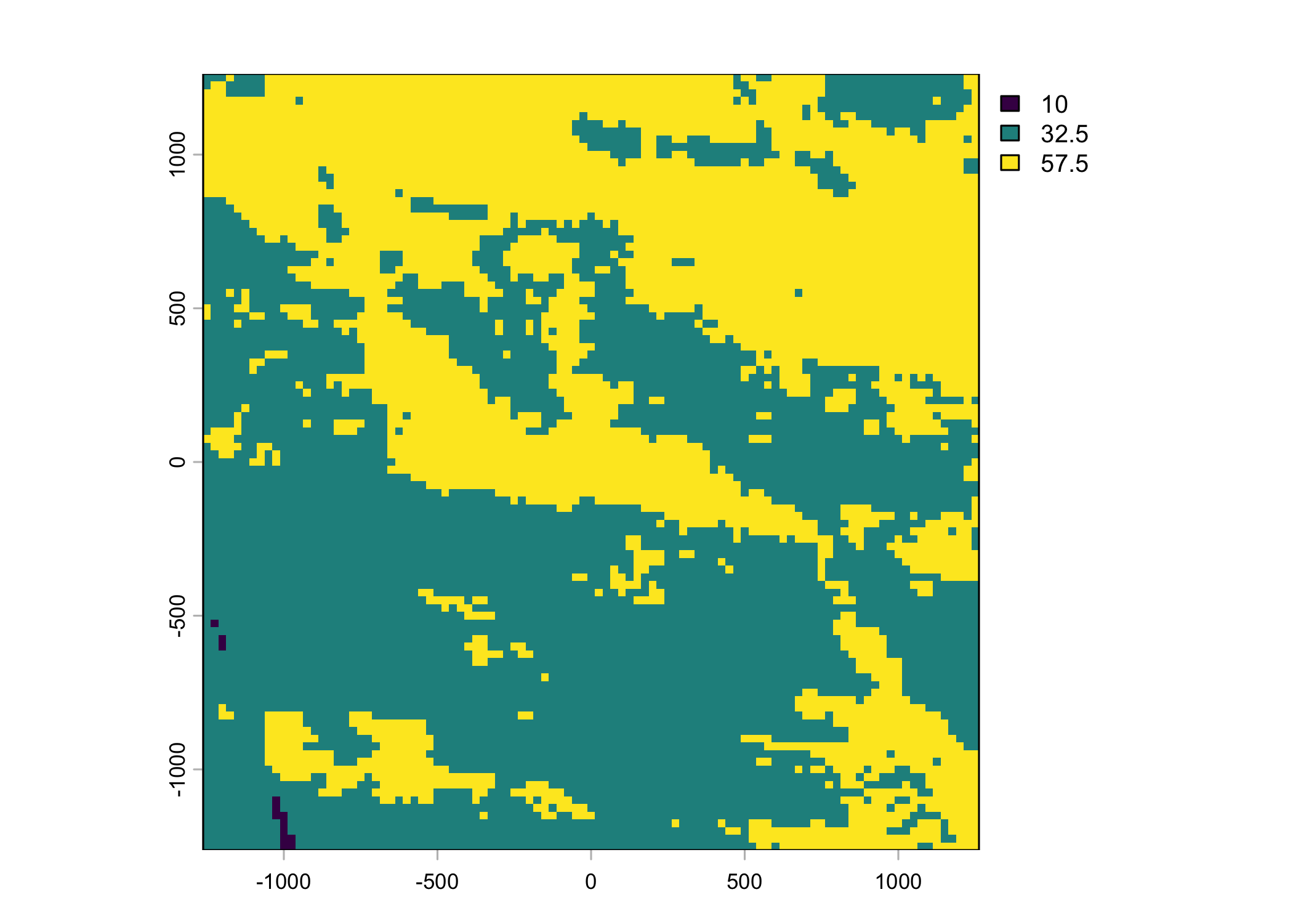
plot(ndvi_projected)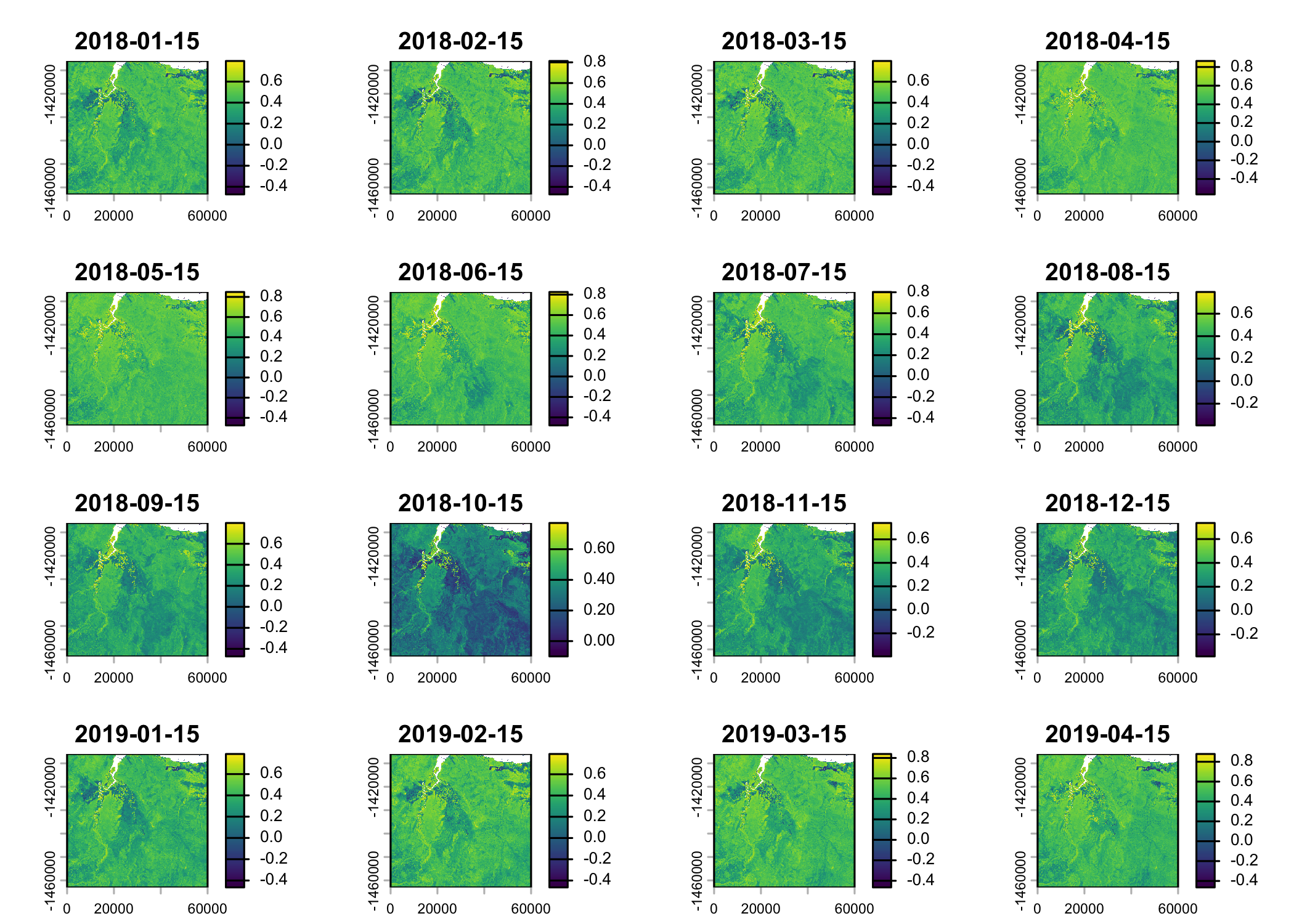
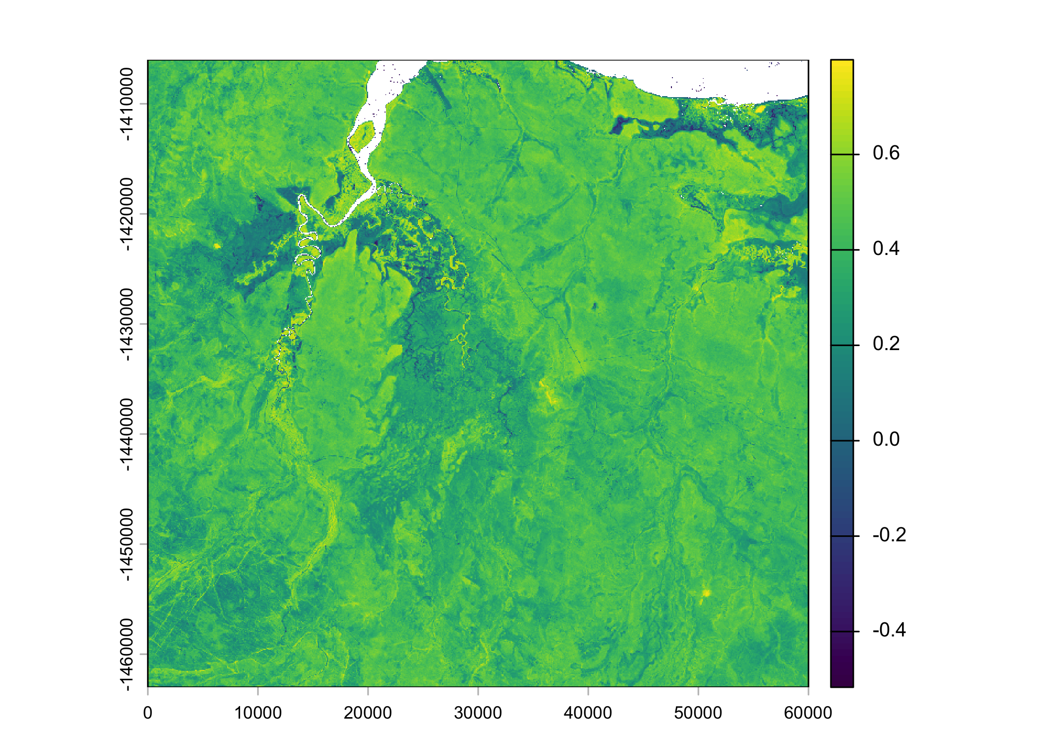
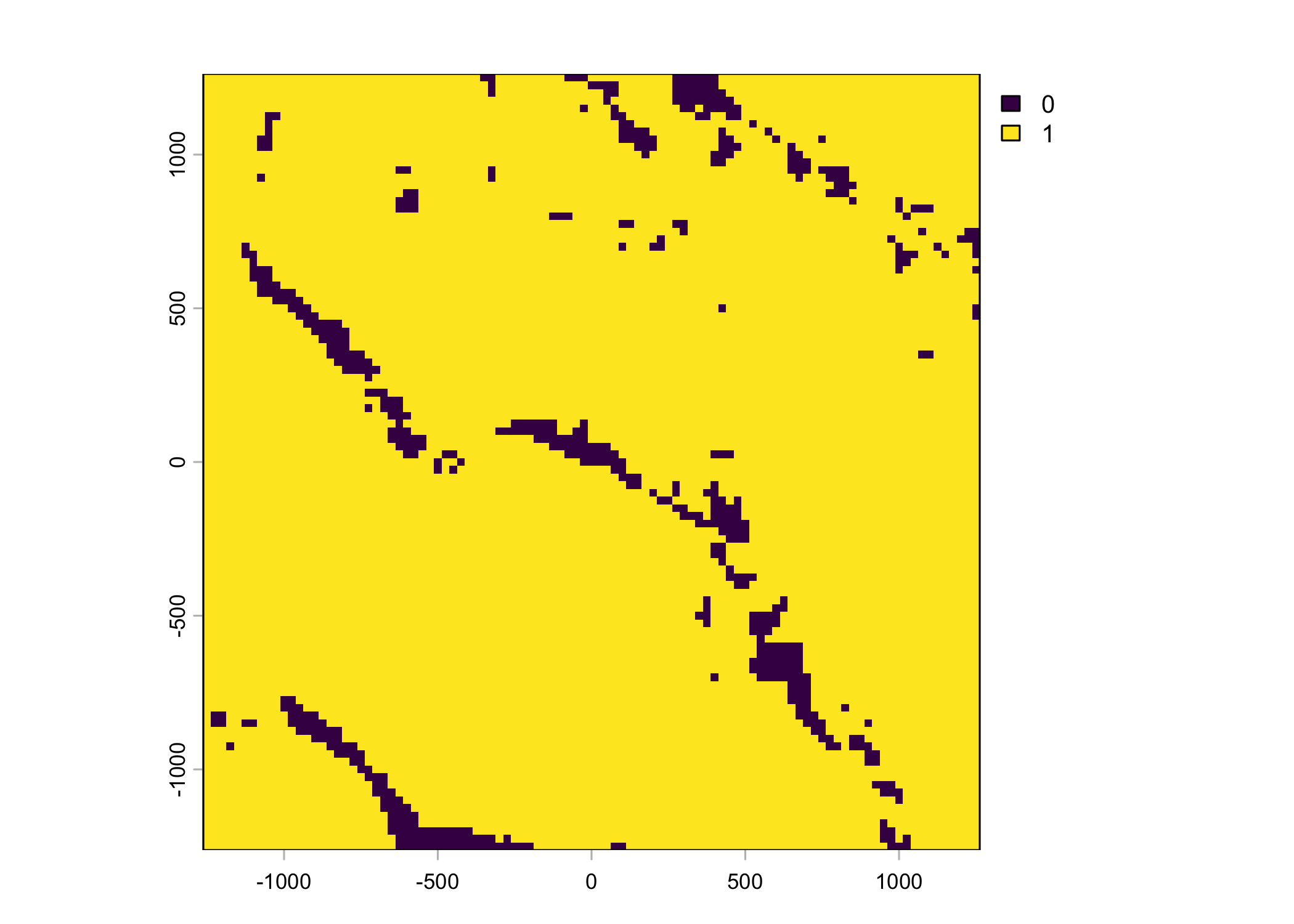
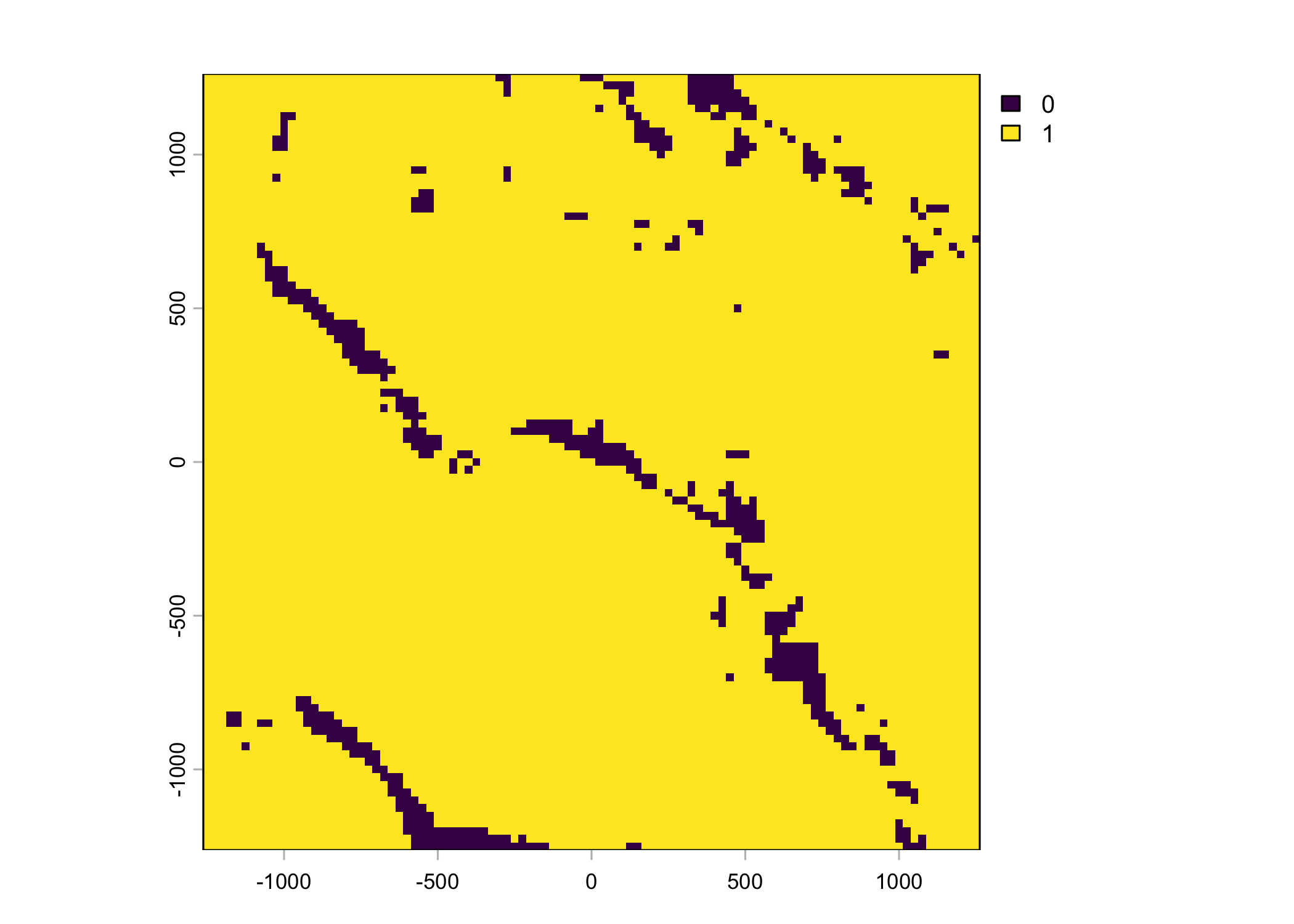
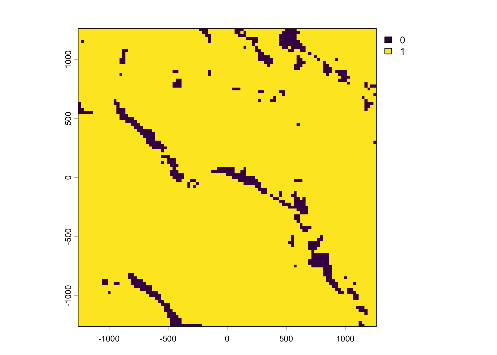
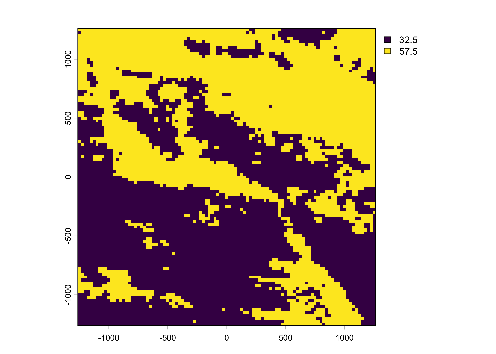
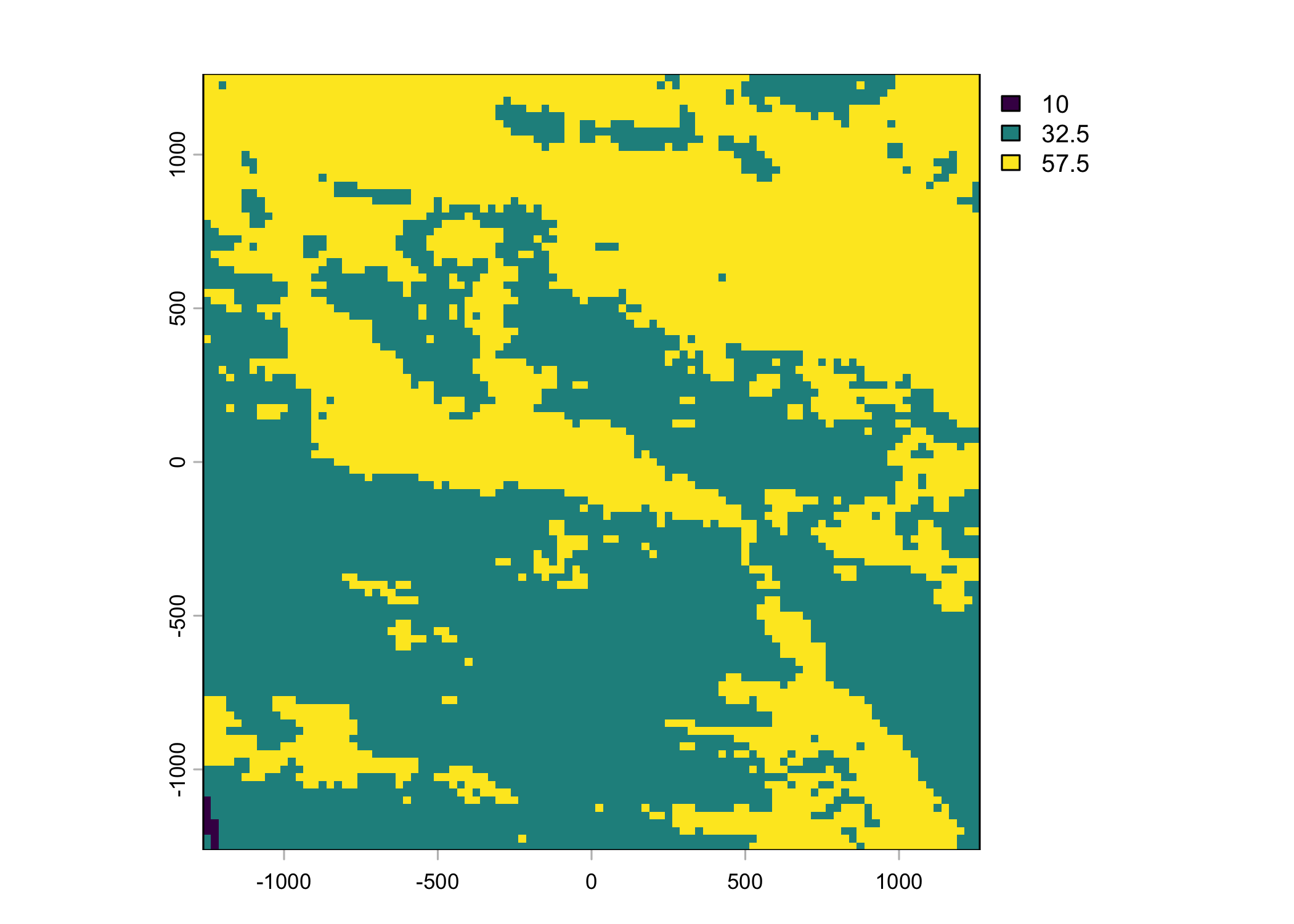
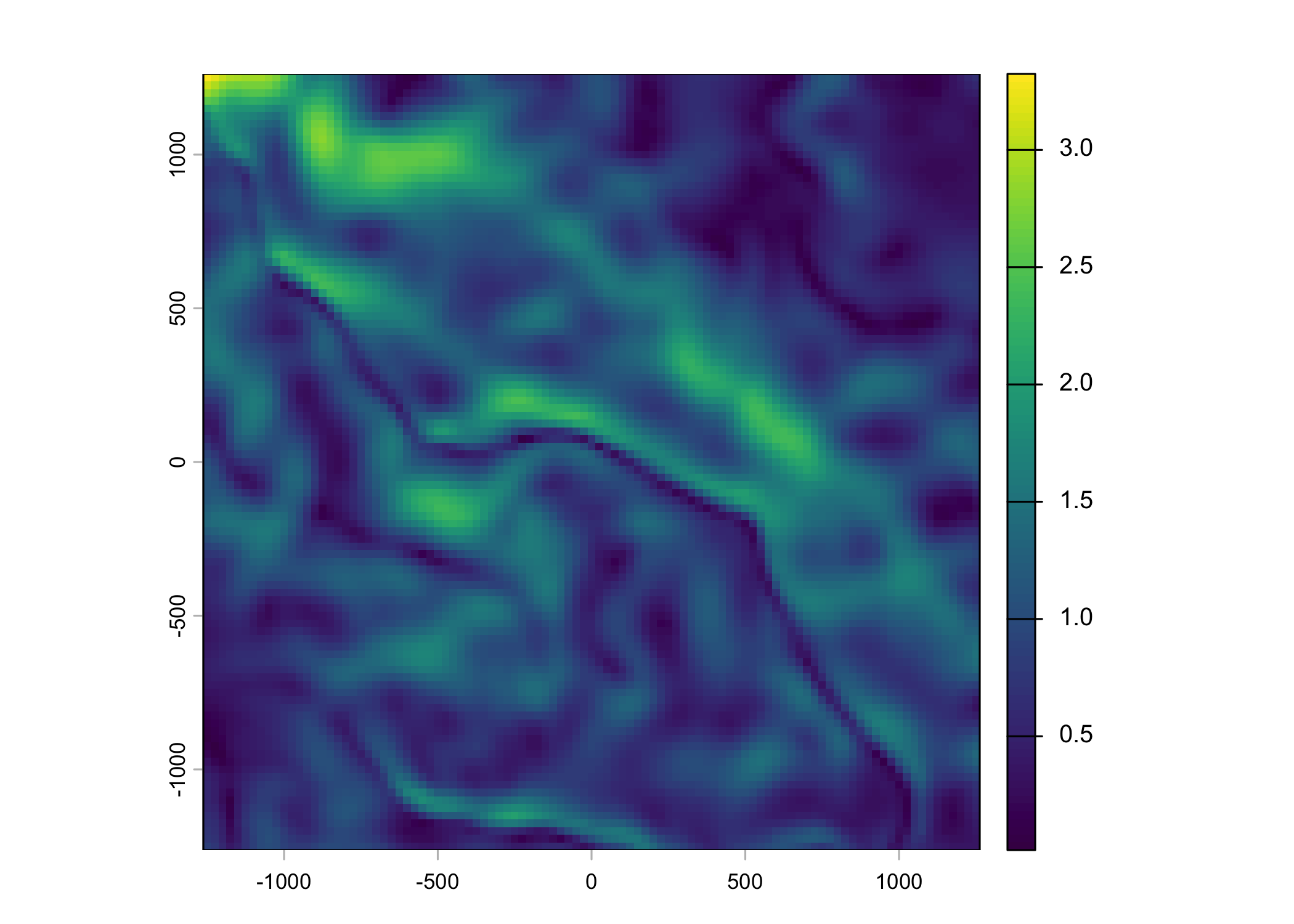
Create some layers for testing the deepSSF package
These will be cropped to the extent of the ID 2005 data. We will also take an average of the NDVI values for simplicity.
Code
Code
# create a buffer around the buffalo 2005 data
buffalo_clean_2005_sf <- buffalo_clean_2005 %>%
st_as_sf(coords = c("lon", "lat"), crs = 4326) %>%
st_transform(crs = 3112)
buffalo_clean_2005_extent <- buffalo_clean_2005_sf %>%
st_buffer(dist = buffer_distance) %>%
st_bbox() %>%
st_as_sfc()
# crop the rasters to the extent of the buffalo 2005 data with the buffer distance
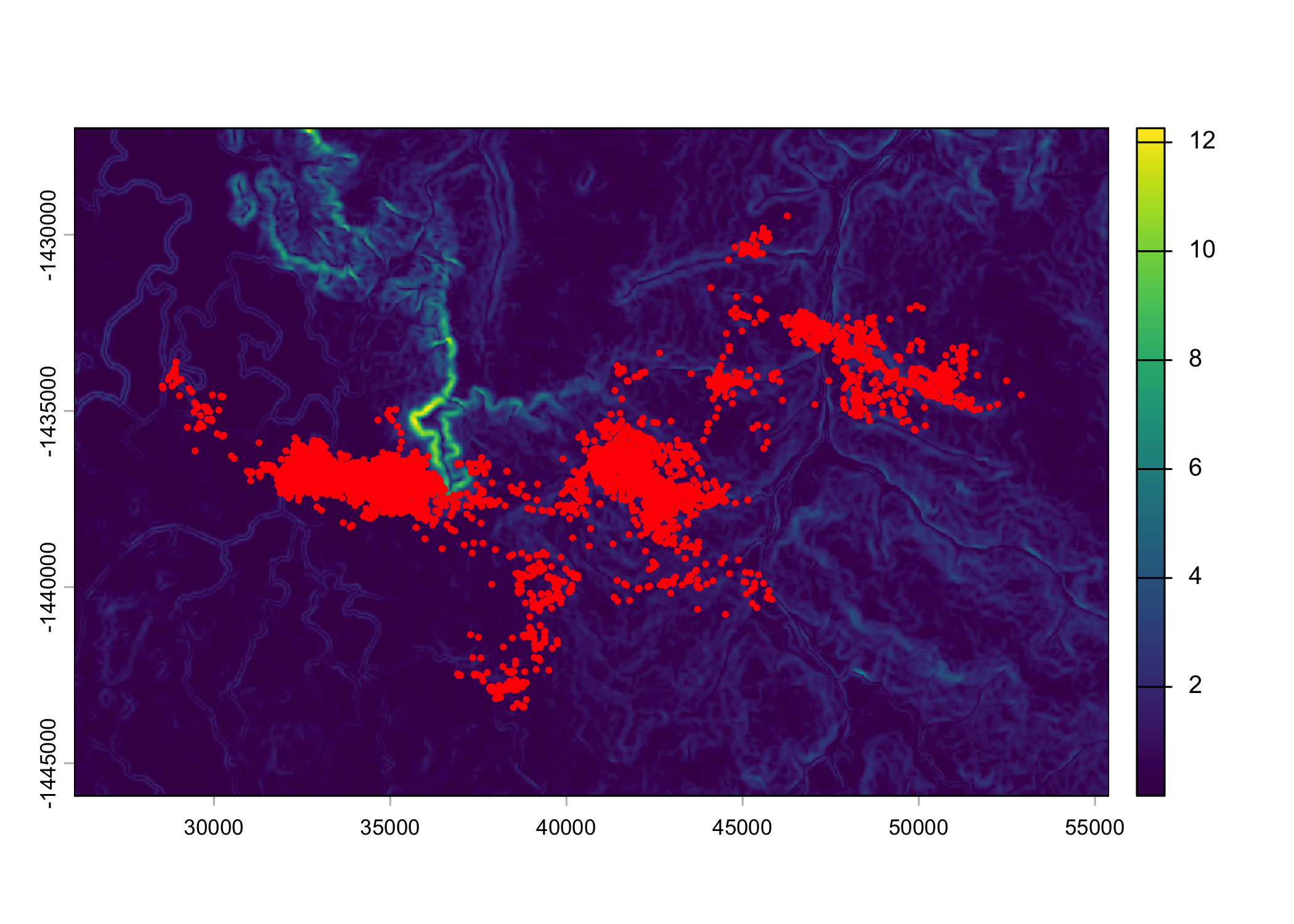
ndvi_2005 <- terra::crop(ndvi_average, buffalo_clean_2005_extent)
slope_2005 <- terra::crop(slope, buffalo_clean_2005_extent)
plot(ndvi_2005)
points(buffalo_clean_2005_sf$geometry, pch = 16, cex = 0.5, col = "red")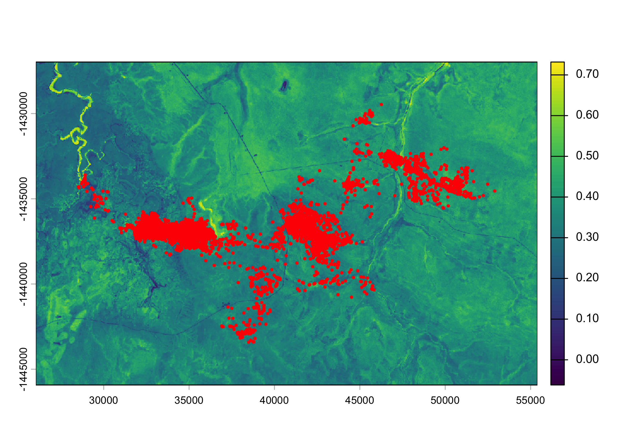
Set up the spatial extent of the local covariates
We calculate the number of cells in each axis, and set the lag between locations. Typically this will just be 1, as we want the next-step to be the target. However, it may be possible to improve model training by using different lags and including the time difference between locations as a covariate. I expect that this would help to predict across different time scales and not be restricted to the time scale that the data was collected at.
Loop over each individual and save the local rasters
This is the main function of the script. It loops over each individual and calculates step level information, such as the location and time of the next step (x2, y2, t2), step length, turning angle, and different time components.
It also determines where to crop the local layers by subtracting and adding the buffer distance from the location of each step. It then crops out the local layers for each step and saves them as a list entry into the data frame.
It then creates a raster stack (with the number of layers equal to the number of steps) for each covariate and saves it as a tif.
For each individual, this will therefore create a csv containing the step level information, and a tif for each covariate containing the local layers for each step.
It takes quite a while to run, around 1 hour per individual in our case, so we will illustrate the function with 10 steps per individual. Uncomment the line specified in the loop to use the full dataset.
Code
# for(i in 1:length(buffalo_ids)) {
for(i in 1:1) { # select just the first ID
buffalo_data <- buffalo_all %>% filter(id == buffalo_ids[i])
# all data for that individual
buffalo_data <- buffalo_data %>% arrange(t_)
# to use a subset of the data for that individual for testing
# COMMENT THIS LINE OUT TO USE THE FULL DATASET
buffalo_data <- buffalo_data %>% arrange(t_) |> slice(1:100)
n_samples <- nrow(buffalo_data)
tic()
buffalo_data_covs <- buffalo_data %>% mutate(
x1_ = x_,
y1_ = y_,
x2_ = lead(x1_, n = hourly_lag, default = NA),
y2_ = lead(y1_, n = hourly_lag, default = NA),
x2_cent = x2_ - x1_,
y2_cent = y2_ - y1_,
t2_ = lead(t_, n = hourly_lag, default = NA),
t_diff = round(difftime(t2_, t_, units = "hours"),0),
# add the minutes as a decimal to the hour, and the hour as a decimal to the day
hour_t1 = round(lubridate::hour(t_) + lubridate::minute(t_)/60,2),
yday_t1 = round(lubridate::yday(t_) + lubridate::hour(t_)/24,2),
hour_t1_sin1 = sin(2*pi*hour_t1/24),
hour_t1_cos1 = cos(2*pi*hour_t1/24),
hour_t1_sin2 = sin(4*pi*hour_t1/24),
hour_t1_cos2 = cos(4*pi*hour_t1/24),
hour_t1_sin3 = sin(6*pi*hour_t1/24),
hour_t1_cos3 = cos(6*pi*hour_t1/24),
yday_t1_sin1 = sin(2*pi*yday_t1/365.25),
yday_t1_cos1 = cos(2*pi*yday_t1/365.25),
yday_t1_sin2 = sin(4*pi*yday_t1/365.25),
yday_t1_cos2 = cos(4*pi*yday_t1/365.25),
yday_t1_sin3 = sin(6*pi*yday_t1/365.25),
yday_t1_cos3 = cos(6*pi*yday_t1/365.25),
# add the minutes as a decimal to the hour, and the hour as a decimal to the day
hour_t2 = round(lubridate::hour(t2_) + lubridate::minute(t2_)/60,2),
hour_t2_sin = sin(2*pi*hour_t2/24),
hour_t2_cos = cos(2*pi*hour_t2/24),
yday_t2 = round(lubridate::yday(t2_) + lubridate::hour(t2_)/24,2),
yday_t2_sin = sin(2*pi*yday_t2/365.25),
yday_t2_cos = cos(2*pi*yday_t2/365.25),
sl = c(sqrt(diff(y_)^2 + diff(x_)^2), NA),
log_sl = log(sl),
bearing = c(atan2(diff(y_), diff(x_)), NA),
bearing_sin = sin(bearing),
bearing_cos = cos(bearing),
ta = c(NA, ifelse(
diff(bearing) > pi, diff(bearing)-(2*pi), ifelse(
diff(bearing) < -pi, diff(bearing)+(2*pi), diff(bearing)))),
cos_ta = cos(ta),
# extent for cropping the spatial covariates
x_min = x_ - buffer,
x_max = x_ + buffer,
y_min = y_ - buffer,
y_max = y_ + buffer,
# crop out and store the local covariates centered on the animal's location
# with an extent set in the previous chunk
) %>% rowwise() %>% mutate(
# the extent needs to be the same for saving the stack of rasters
extent_00centre = list(ext(x_min - x_, x_max - x_, y_min - y_, y_max - y_)),
# NDVI
ndvi_index = which.min(abs(difftime(t_, terra::time(ndvi_projected)))),
ndvi_cent = list({
ndvi_cent = crop(ndvi_projected[[ndvi_index]], ext(x_min, x_max, y_min, y_max))
ext(ndvi_cent) <- extent_00centre
ndvi_cent
}),
# herbaceous vegetation
veg_herby_cent = list({
veg_herby_cent = crop(veg_herby, ext(x_min, x_max, y_min, y_max))
ext(veg_herby_cent) <- extent_00centre
veg_herby_cent
}),
# canopy cover
canopy_cover_cent = list({
canopy_cover_cent = crop(canopy_cover, ext(x_min, x_max, y_min, y_max))
ext(canopy_cover_cent) <- extent_00centre
canopy_cover_cent
}),
# slope
slope_cent = list({
slope_cent <- crop(slope, ext(x_min, x_max, y_min, y_max))
ext(slope_cent) <- extent_00centre
slope_cent
}),
# presence (next-step)
pres_template = list({
pres_template <- crop(slope, ext(x_min, x_max, y_min, y_max))
pres_template
}),
# Strict within cell method
points_vect_cent_x2_within_cell = list(terra::vect(cbind(x2_, y2_), type = "points", crs = "EPSG:3112")),
pres_cent_x2_within_cell = list({
pres_cent_x2_within_cell <- rasterize(points_vect_cent_x2_within_cell, pres_template, background=0)
ext(pres_cent_x2_within_cell) <- extent_00centre
pres_cent_x2_within_cell
})
) %>% ungroup() # to remove the 'rowwise' class
toc()
# remove steps that fall outside of the local spatial extent
buffalo_data_covs <- buffalo_data_covs %>%
filter(x2_cent > -buffer & x2_cent < buffer & y2_cent > -buffer & y2_cent < buffer) %>%
drop_na(ta)
# remove the columns that are no longer needed
buffalo_data_df <- buffalo_data_covs %>%
dplyr::select(
-extent_00centre,
-ndvi_cent,
-veg_herby_cent,
-canopy_cover_cent,
-slope_cent,
-pres_template,
-points_vect_cent_x2_within_cell,
-pres_cent_x2_within_cell)
# save the data
write_csv(buffalo_data_df, paste0("buffalo_local_data_id/buffalo_temporal_cont_", buffalo_ids[i],
"_data_df_lag_", hourly_lag, "hr_n", n_samples, ".csv"))
# saving the raster objects
rast(buffalo_data_covs$ndvi_cent) %>%
writeRaster(paste0("buffalo_local_layers_id/buffalo_", buffalo_ids[i], "_ndvi_cent",
nxn_cells, "x", nxn_cells, "_lag_", hourly_lag, "hr_n", n_samples, ".tif"),
overwrite = T)
rast(buffalo_data_covs$veg_herby_cent) %>%
writeRaster(paste0("buffalo_local_layers_id/buffalo_", buffalo_ids[i], "_herby_cent",
nxn_cells, "x", nxn_cells, "_lag_", hourly_lag, "hr_n", n_samples, ".tif"),
overwrite = T)
rast(buffalo_data_covs$canopy_cover_cent) %>%
writeRaster(paste0("buffalo_local_layers_id/buffalo_", buffalo_ids[i], "_canopy_cent",
nxn_cells, "x", nxn_cells, "_lag_", hourly_lag, "hr_n", n_samples, ".tif"),
overwrite = T)
rast(buffalo_data_covs$slope_cent) %>%
writeRaster(paste0("buffalo_local_layers_id/buffalo_", buffalo_ids[i], "_slope_cent",
nxn_cells, "x", nxn_cells, "_lag_", hourly_lag, "hr_n", n_samples, ".tif"),
overwrite = T)
rast(buffalo_data_covs$pres_cent_x2_within_cell) %>%
writeRaster(paste0("buffalo_local_layers_id/within_cell_buffalo_", buffalo_ids[i], "_pres_cent",
nxn_cells, "x", nxn_cells, "_lag_", hourly_lag, "hr_n", n_samples, ".tif"),
overwrite = T)
}6.431 sec elapsedCheck the outputs
Plot a subset of the local covariates

Code
Warning: Unknown or uninitialised column: `pres_cent_x1`.Code


To save the object with all of the local covariates
To save some plots
Code
# for(i in 1:n_plots) {
# png(filename = paste0("ndvi_cent_", i, ".png"),
# width = 150, height = 150, units = "mm", res = 600)
# terra::plot(buffalo_data_covs$ndvi_cent[[i]])
# dev.off()
# }
#
# # for the pres layers
# for(i in 1:n_plots) {
#
# # change the 0 values to NA
# layer <- buffalo_data_covs$pres_cent[[i]]
# layer[layer == 0] <- 0.5
#
# ndvi_layer <- buffalo_data_covs$ndvi_cent[[i]]
# new_layer <- layer*ndvi_layer
#
# # save the plot
# png(filename = paste0("pres_cent_", i, ".png"),
# width = 150, height = 150, units = "mm", res = 600)
# terra::plot(new_layer)
# dev.off()
# }
#
#
# # other plots
#
# n_plots <- 1
#
# for(i in 1:n_plots) {
# png(filename = paste0("veg_herby_cent_", i, ".png"),
# width = 150, height = 150, units = "mm", res = 600)
# terra::plot(buffalo_data_covs$veg_herby_cent[[i]])
# dev.off()
# }
#
# for(i in 1:n_plots) {
# png(filename = paste0("canopy_cover_cent_", i, ".png"),
# width = 150, height = 150, units = "mm", res = 600)
# terra::plot(buffalo_data_covs$canopy_cover_cent[[i]])
# dev.off()
# }
#
# for(i in 1:n_plots) {
# png(filename = paste0("slope_cent_", i, ".png"),
# width = 150, height = 150, units = "mm", res = 600)
# terra::plot(buffalo_data_covs$slope_cent[[i]])
# dev.off()
# }Plot the step lengths and turning angles
Code
Code
# ggsave("outputs/step_length.png", height = 60, width = 120, units = "mm", dpi = 600)
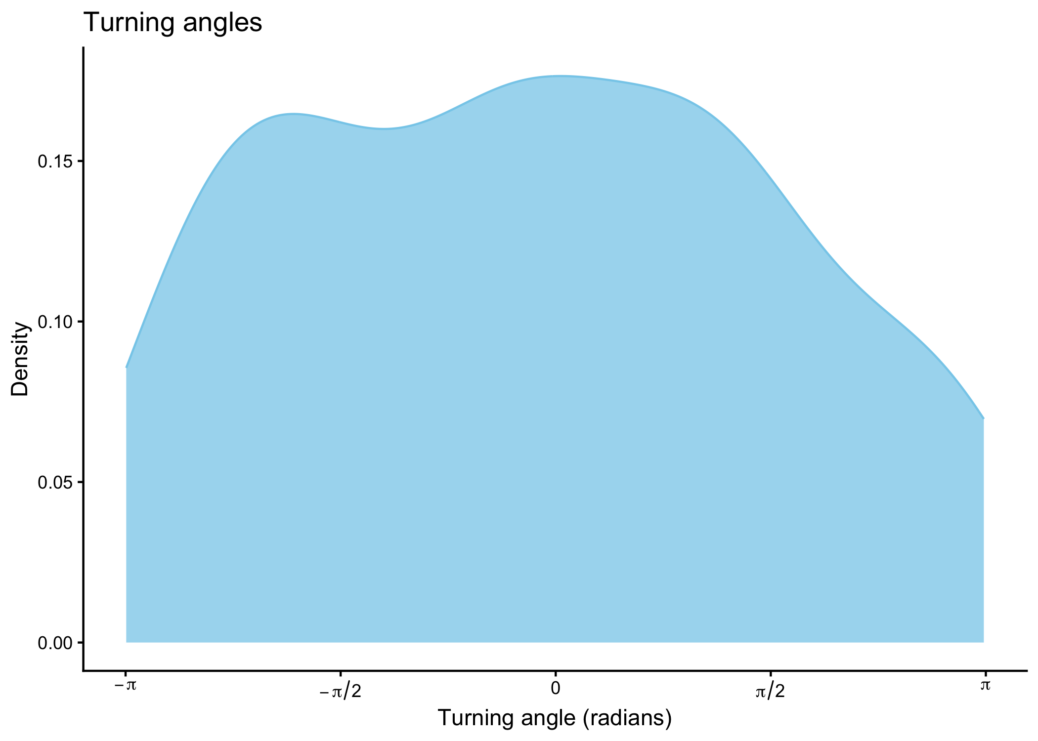
# plot turning angles
buffalo_data_covs %>% ggplot() +
geom_density(aes(x = ta),
fill = "skyblue", colour = "skyblue", alpha = 0.75) +
scale_x_continuous("Turning angle (radians)",
breaks = c(-pi, -pi/2, 0, pi/2, pi),
labels = c(expression(-pi), expression(-pi/2), "0", expression(pi/2), expression(pi))
) +
scale_y_continuous("Density") +
ggtitle("Turning angles") +
theme_classic()