# Create directory for saving prediction images
os.makedirs(f'{output_dir}/prediction_images', exist_ok=True)
# Start at 1 so the bearing at t - 1 is available
for i in range(1, n_samples):
sample = test_data.iloc[i]
# Current location (x1, y1)
x = sample['x1_']
y = sample['y1_']
# Convert geographic coordinates to pixel coordinates
px, py = ~raster_transform * (x, y)
# Next step location (x2, y2)
x2 = sample['x2_']
y2 = sample['y2_']
# Convert geographic coordinates to pixel coordinates
px2, py2 = ~raster_transform * (x2, y2)
# The difference in x and y coordinates
d_x = x2 - x
d_y = y2 - y
# print('d_x and d_y are ', d_x, d_y) # Debugging
# Temporal covariates for t1
hour_t1_sin1 = sample['hour_t1_sin1']
hour_t1_cos1 = sample['hour_t1_cos1']
hour_t1_sin2 = sample['hour_t1_sin2']
hour_t1_cos2 = sample['hour_t1_cos2']
yday_t1_sin1 = sample['yday_t1_sin1']
yday_t1_cos1 = sample['yday_t1_cos1']
yday_t1_sin2 = sample['yday_t1_sin2']
yday_t1_cos2 = sample['yday_t1_cos2']
# Bearing of previous step (t - 1)
bearing = sample['bearing_tm1']
# Hour of the day (for saving the plot)
hour_t2 = sample['hour_t2']
# Day of the year
yday = sample['yday_t2']
# Convert day of the year to month index
month_index = day_to_month_index(yday)
# print(month_index)
# For sentinel 2 data
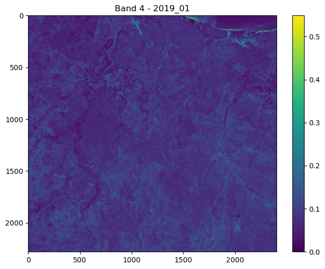
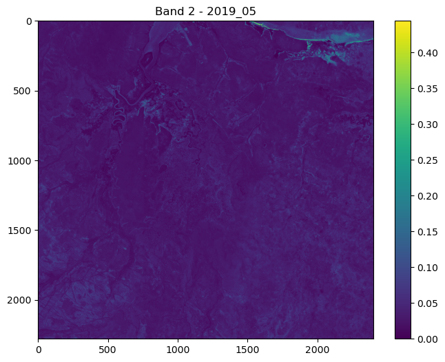
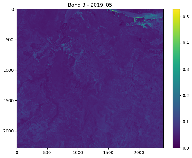
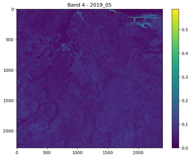
selected_month = f'2019_{month_index:02d}'
# Get the Sentinel-2 layers for the selected month
s2_data = data_dict[selected_month]
# Convert the Sentinel-2 data from a NumPy array to a PyTorch tensor
s2_tensor = torch.from_numpy(s2_data)
s2_tensor = s2_tensor.float() # Ensure the tensor is of type float
# print(s2_tensor.shape)
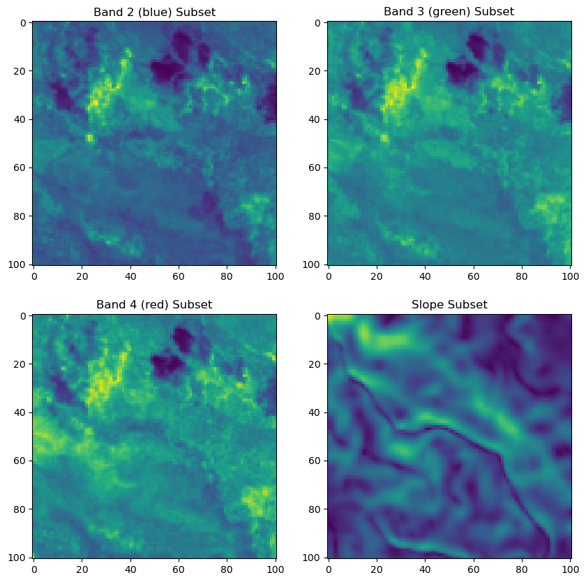
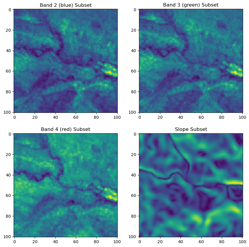
# Crop out the Sentinel-2 subsets at the location of x1, y1
s2_b1_subset, origin_x, origin_y = subset_function(s2_tensor[0,:,:], x, y, window_size, raster_transform)
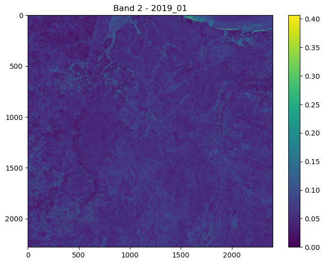
s2_b2_subset, origin_x, origin_y = subset_function(s2_tensor[1,:,:], x, y, window_size, raster_transform)
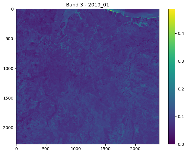
s2_b3_subset, origin_x, origin_y = subset_function(s2_tensor[2,:,:], x, y, window_size, raster_transform)
s2_b4_subset, origin_x, origin_y = subset_function(s2_tensor[3,:,:], x, y, window_size, raster_transform)
s2_b5_subset, origin_x, origin_y = subset_function(s2_tensor[4,:,:], x, y, window_size, raster_transform)
s2_b6_subset, origin_x, origin_y = subset_function(s2_tensor[5,:,:], x, y, window_size, raster_transform)
s2_b7_subset, origin_x, origin_y = subset_function(s2_tensor[6,:,:], x, y, window_size, raster_transform)
s2_b8_subset, origin_x, origin_y = subset_function(s2_tensor[7,:,:], x, y, window_size, raster_transform)
s2_b8a_subset, origin_x, origin_y = subset_function(s2_tensor[8,:,:], x, y, window_size, raster_transform)
s2_b9_subset, origin_x, origin_y = subset_function(s2_tensor[9,:,:], x, y, window_size, raster_transform)
s2_b11_subset, origin_x, origin_y = subset_function(s2_tensor[10,:,:], x, y, window_size, raster_transform)
s2_b12_subset, origin_x, origin_y = subset_function(s2_tensor[11,:,:], x, y, window_size, raster_transform)
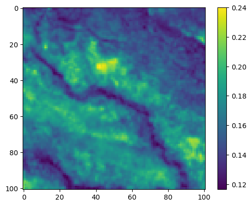
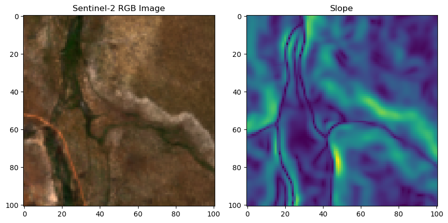
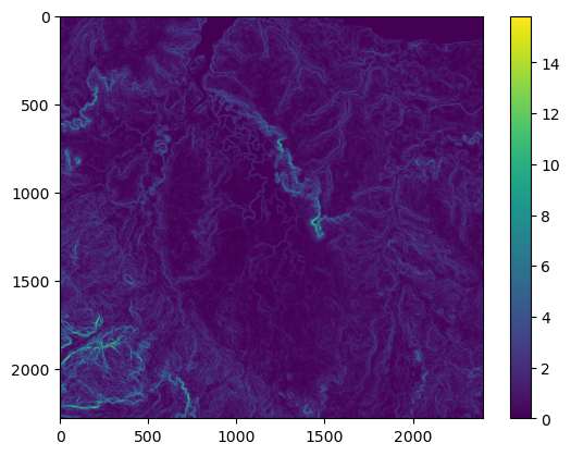
# Crop out the slope subset at the location of x1, y1
slope_subset, origin_x, origin_y = subset_function(slope_landscape_norm, x, y, window_size, raster_transform)
# Location of the next step in local pixel coordinates
px2_subset = px2 - origin_x
py2_subset = py2 - origin_y
# print('px2_subset and py2_subset are ', px2_subset, py2_subset) # Debugging
# Stack the channels along a new axis
x1 = torch.stack([s2_b1_subset,
s2_b2_subset,
s2_b3_subset,
s2_b4_subset,
s2_b5_subset,
s2_b6_subset,
s2_b7_subset,
s2_b8_subset,
s2_b8a_subset,
s2_b9_subset,
s2_b11_subset,
s2_b12_subset,
slope_subset], dim=0)
# Add a batch dimension (required to be the correct dimension for the model)
x1 = x1.unsqueeze(0).to(device)
# print(x1.shape)
# Temporal covariates for t1
hour_t1_sin1_tensor = torch.tensor(hour_t1_sin1).float()
hour_t1_cos1_tensor = torch.tensor(hour_t1_cos1).float()
hour_t1_sin2_tensor = torch.tensor(hour_t1_sin2).float()
hour_t1_cos2_tensor = torch.tensor(hour_t1_cos2).float()
yday_t1_sin1_tensor = torch.tensor(yday_t1_sin1).float()
yday_t1_cos1_tensor = torch.tensor(yday_t1_cos1).float()
yday_t1_sin2_tensor = torch.tensor(yday_t1_sin2).float()
yday_t1_cos2_tensor = torch.tensor(yday_t1_cos2).float()
# Stack tensors
x2 = torch.stack((hour_t1_sin1_tensor.unsqueeze(0),
hour_t1_cos1_tensor.unsqueeze(0),
hour_t1_sin2_tensor.unsqueeze(0),
hour_t1_cos2_tensor.unsqueeze(0),
yday_t1_sin1_tensor.unsqueeze(0),
yday_t1_cos1_tensor.unsqueeze(0),
yday_t1_sin2_tensor.unsqueeze(0),
yday_t1_cos2_tensor.unsqueeze(0)),
dim=1).to(device)
# print(x2)
# print(x2.shape)
# put bearing in the correct dimension (batch_size, 1)
bearing = torch.tensor(bearing).float().unsqueeze(0).unsqueeze(0).to(device)
# print(bearing)
# print(bearing.shape)
# -------------------------------------------------------------------------
# Run the model
# -------------------------------------------------------------------------
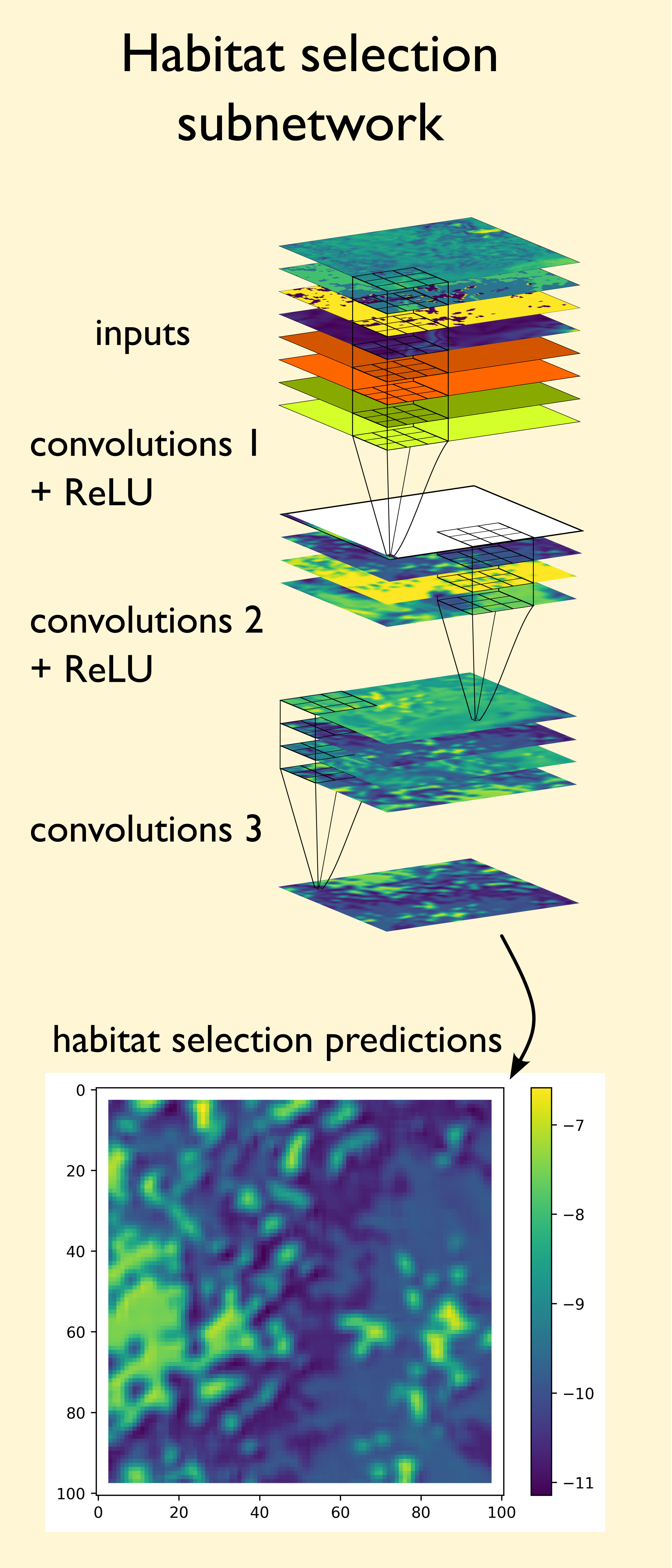
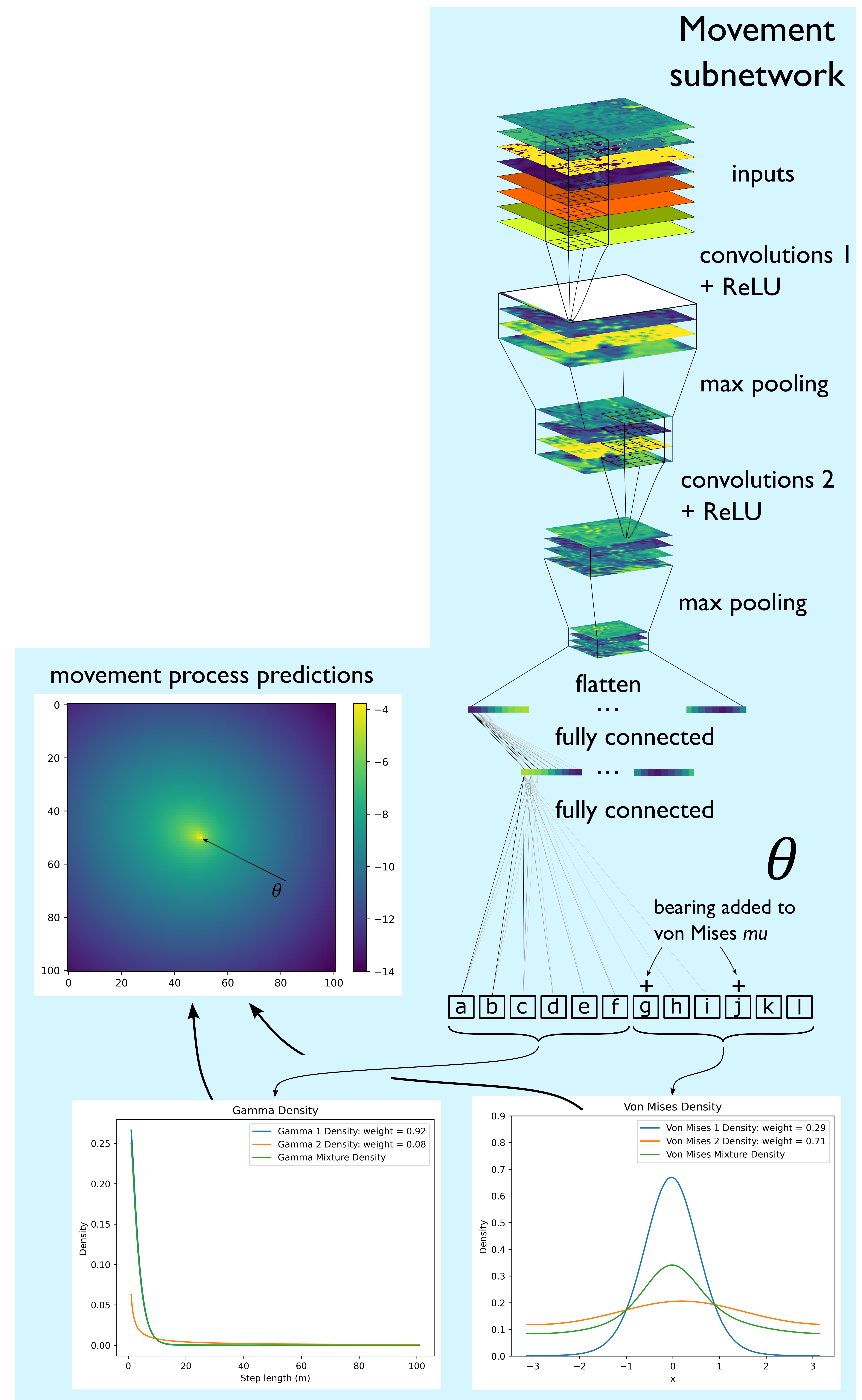
model_output = model((x1, x2, bearing))
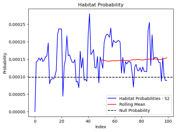
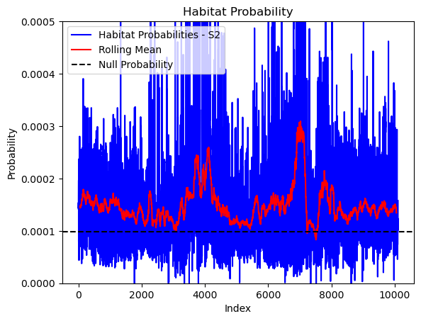
# -------------------------------------------------------------------------
# Habitat selection probability
# -------------------------------------------------------------------------
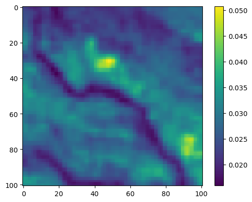
hab_density = model_output.detach().cpu().numpy()[0,:,:,0]
hab_density_exp = np.exp(hab_density)
# Normalise the probability surface to sum to 1
hab_density_exp_norm = hab_density_exp / np.sum(hab_density_exp)
# print(np.sum(hab_density_exp_norm)) # Should be 1
# Store the probability of habitat selection at the location of x2, y2
# These probabilities are normalised in the model function
habitat_probs[i] = hab_density_exp_norm[(int(py2_subset), int(px2_subset))]
# print('Habitat probability value = ', habitat_probs[i])
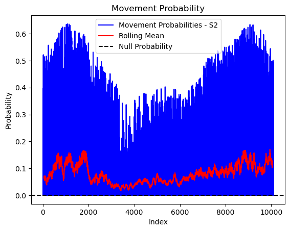
# -------------------------------------------------------------------------
# Movement probability
# -------------------------------------------------------------------------
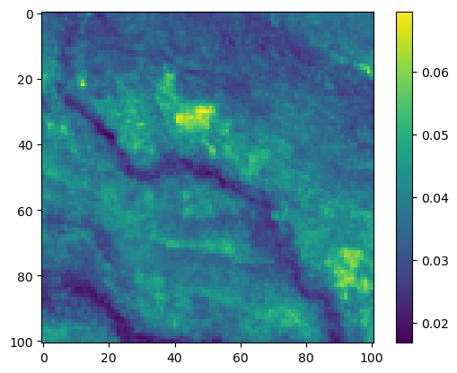
move_density = model_output.detach().cpu().numpy()[0,:,:,1]
move_density_exp = np.exp(move_density)
# Normalise the probability surface to sum to 1
move_density_exp_norm = move_density_exp / np.sum(move_density_exp)
# print(np.sum(move_density_exp_norm)) # Should be 1
# Store the movement probability at the location of x2, y2
# These probabilities are normalised in the model function
move_probs[i] = move_density_exp_norm[(int(py2_subset), int(px2_subset))]
# print('Movement probability value = ', move_probs[i])
# -------------------------------------------------------------------------
# Next step probability
# -------------------------------------------------------------------------
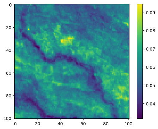
step_density = hab_density + move_density
step_density_exp = np.exp(step_density)
# print('Sum of step density exp = ', np.sum(step_density_exp)) # Won't be 1
step_density_exp_norm = step_density_exp / np.sum(step_density_exp)
# print('Sum of step density exp norm = ', np.sum(step_density_exp_norm)) # Should be 1
# Extract the value of the covariates at the location of x2, y2
next_step_probs[i] = step_density_exp_norm[(int(py2_subset), int(px2_subset))]
# print('Next-step probability value = ', next_step_probs[i])
# -------------------------------------------------------------------------
# Plot the next-step predictions
# -------------------------------------------------------------------------
# Plot the first few probability surfaces - change the condition to i < n_steps to plot all
if i < 51:
# Mask out bordering cells
hab_density_mask = hab_density * x_mask * y_mask
move_density_mask = move_density * x_mask * y_mask
step_density_mask = step_density * x_mask * y_mask
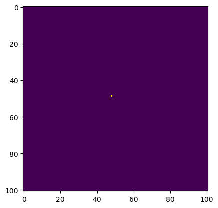
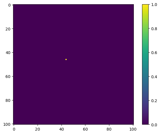
# Create a mask for the next step
next_step_mask = np.ones_like(hab_density)
next_step_mask[int(py2_subset), int(px2_subset)] = -np.inf
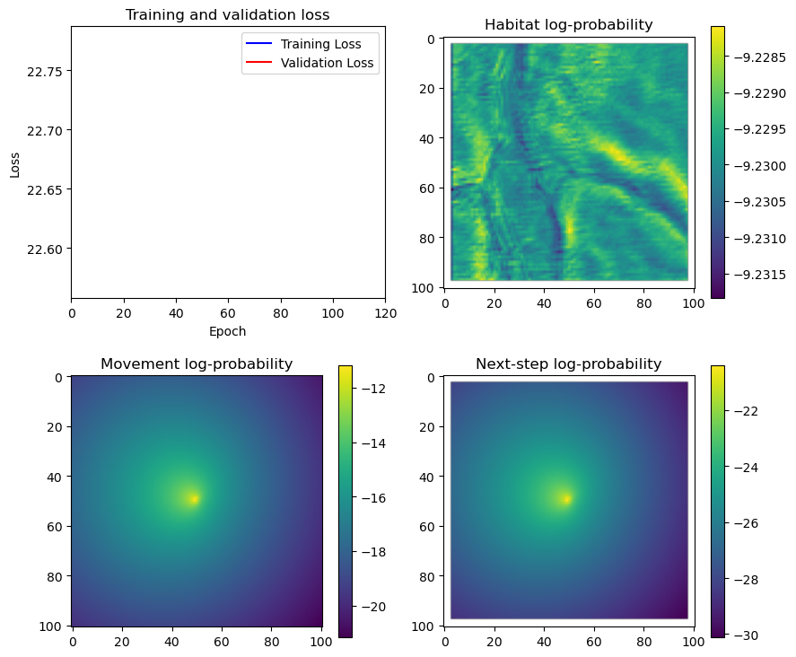
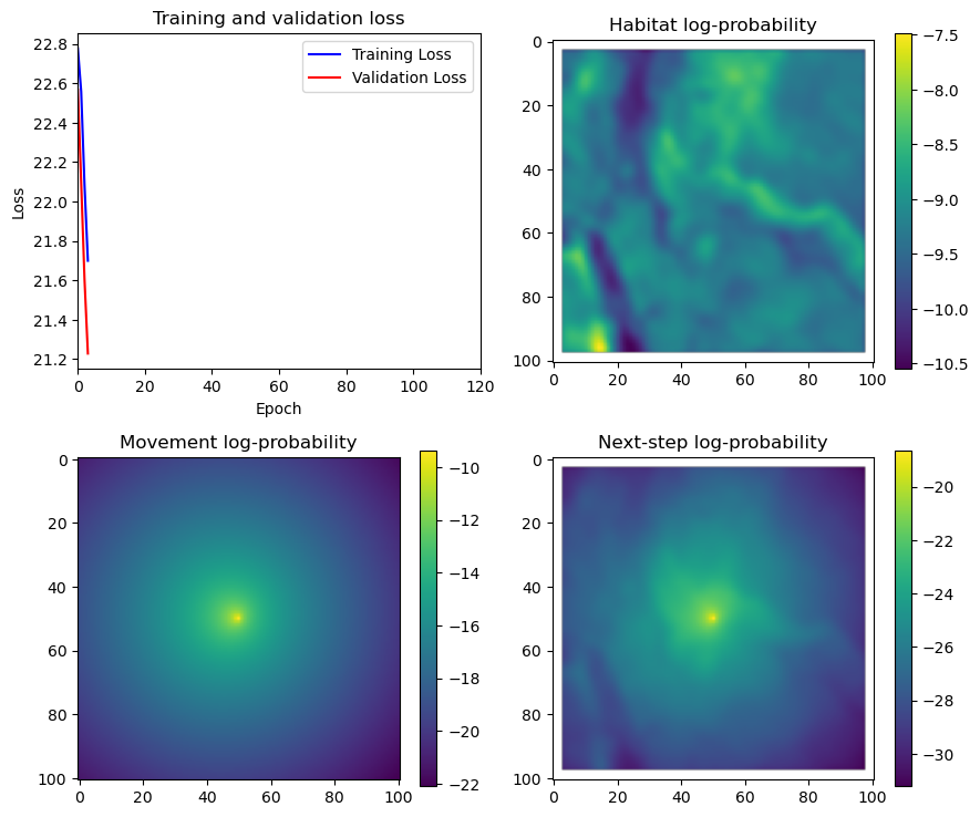
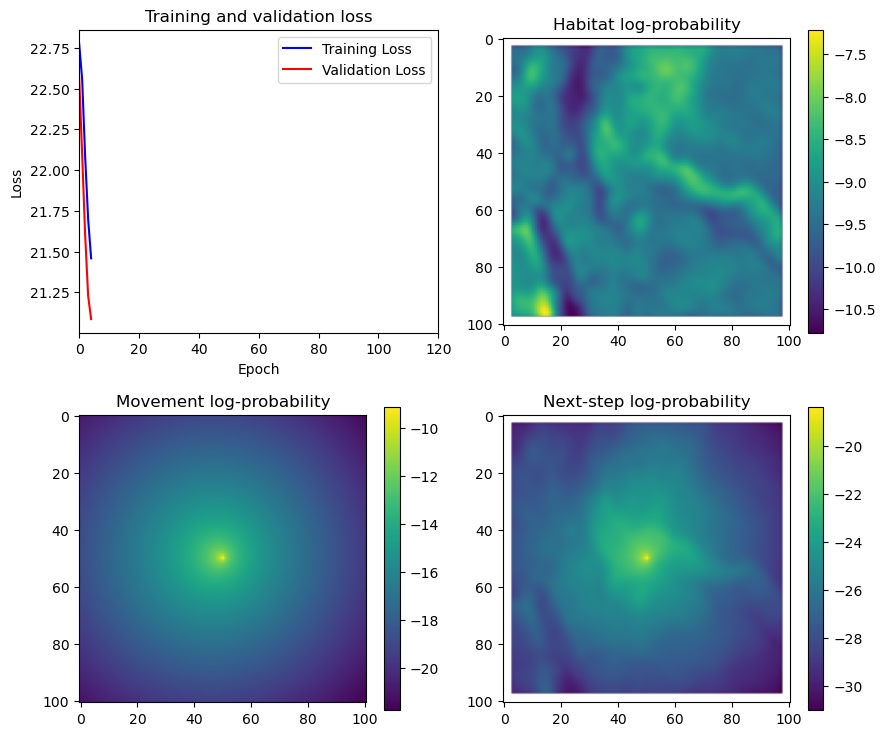
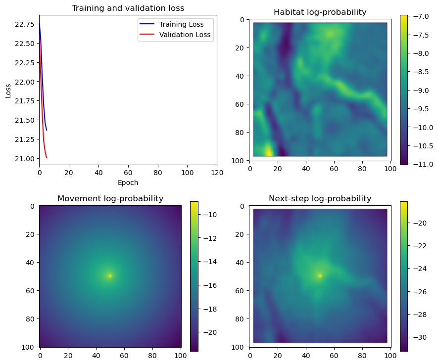
# Plot the outputs
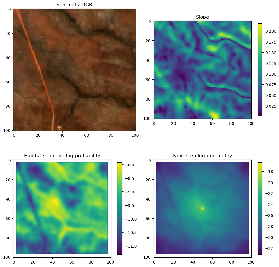
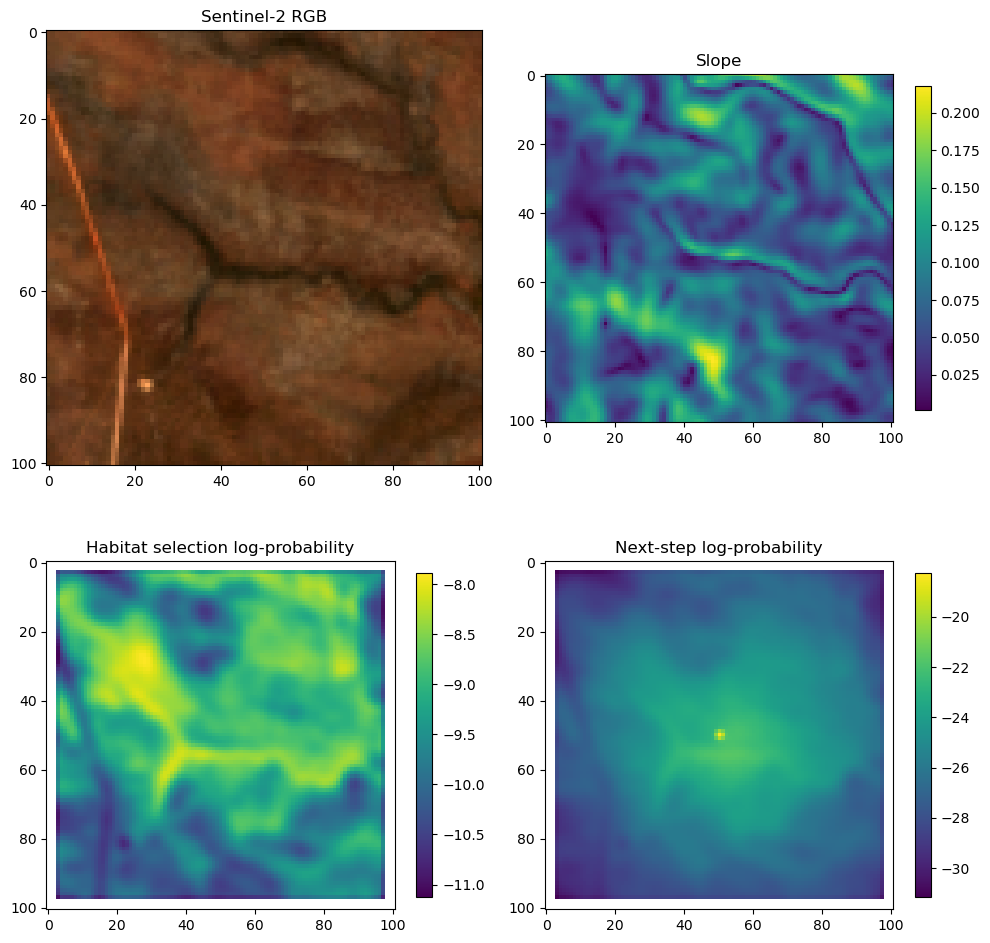
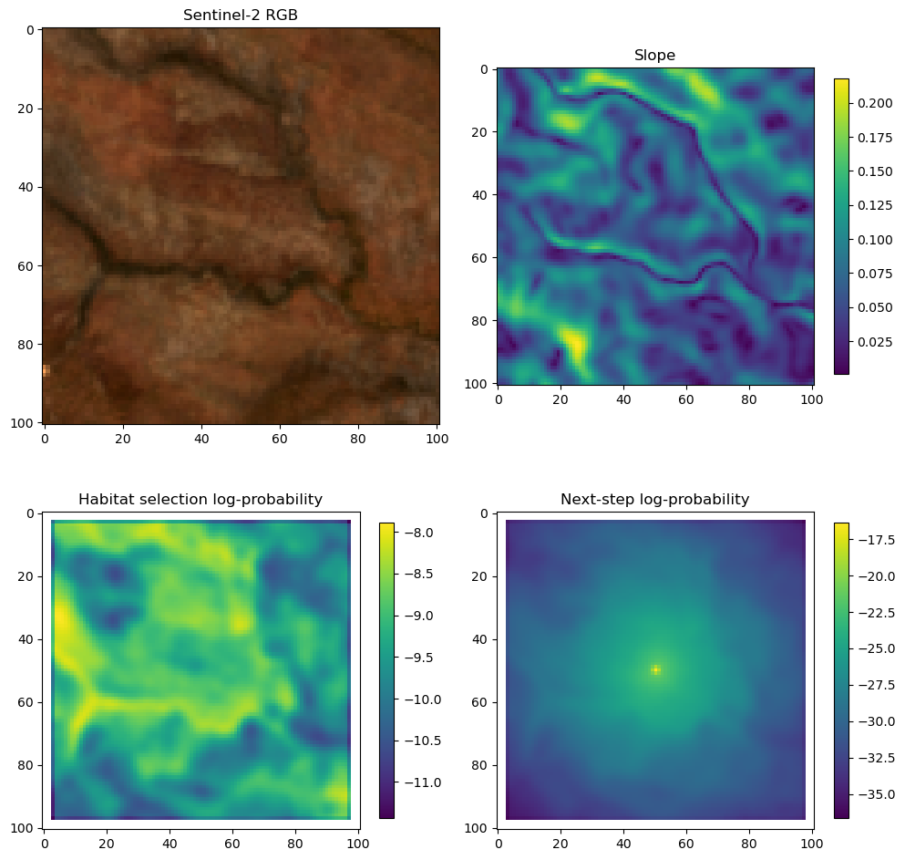
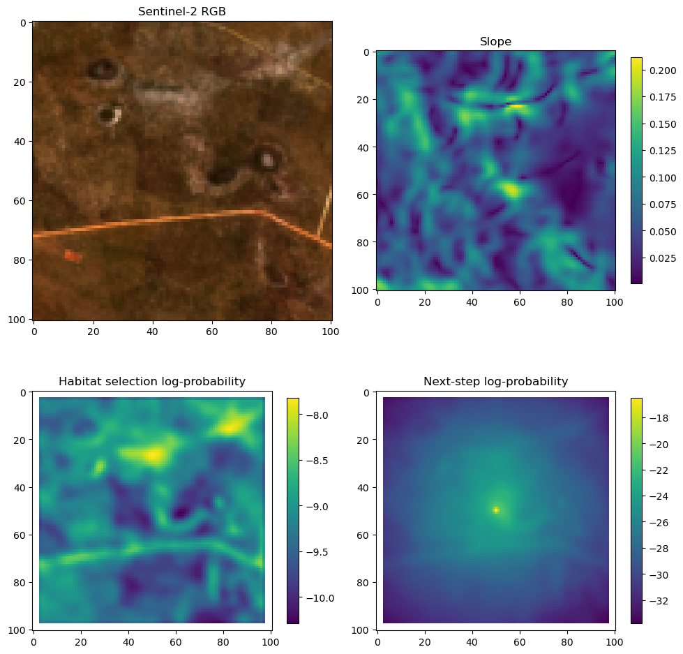
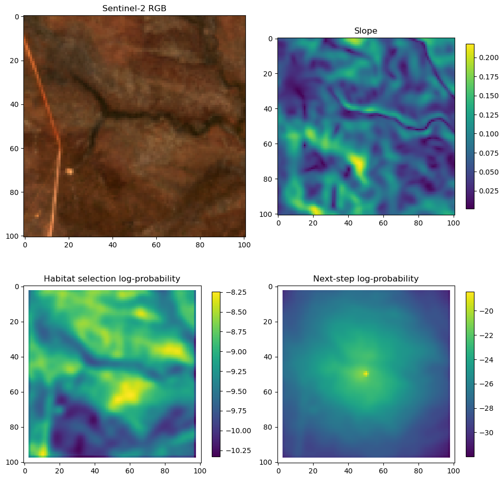
fig_out, axs_out = plt.subplots(2, 2, figsize=(10, 8))
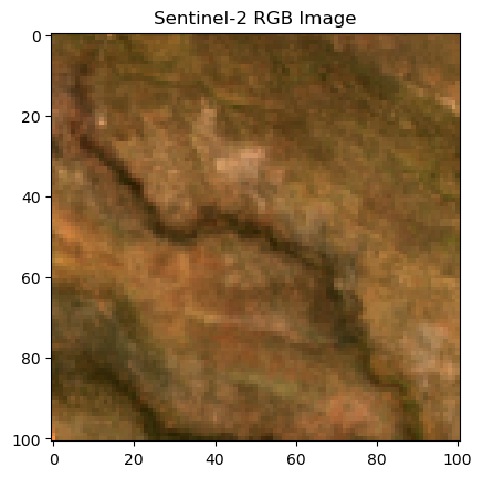
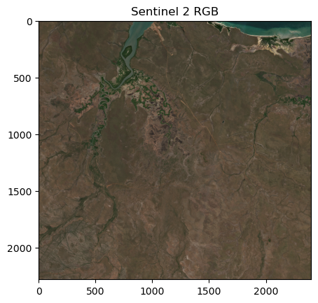
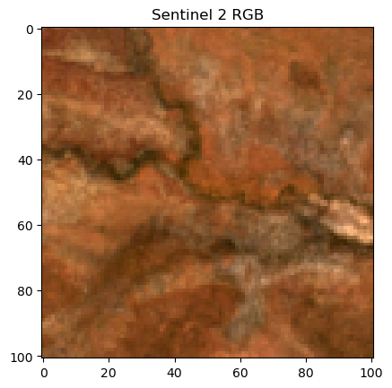
# RGB for plotting
# pull out the RGB bands
r_band = s2_b4_subset.detach().numpy()
g_band = s2_b3_subset.detach().numpy()
b_band = s2_b2_subset.detach().numpy()
# Stack the bands along a new axis
rgb_image = np.stack([r_band, g_band, b_band], axis=-1)
# Normalize to the range [0, 1] for display
rgb_image = (rgb_image - rgb_image.min()) / (rgb_image.max() - rgb_image.min())
# Plot s2_b2
im1 = axs_out[0, 0].imshow(rgb_image)
axs_out[0, 0].set_title('Sentinel 2 RGB')
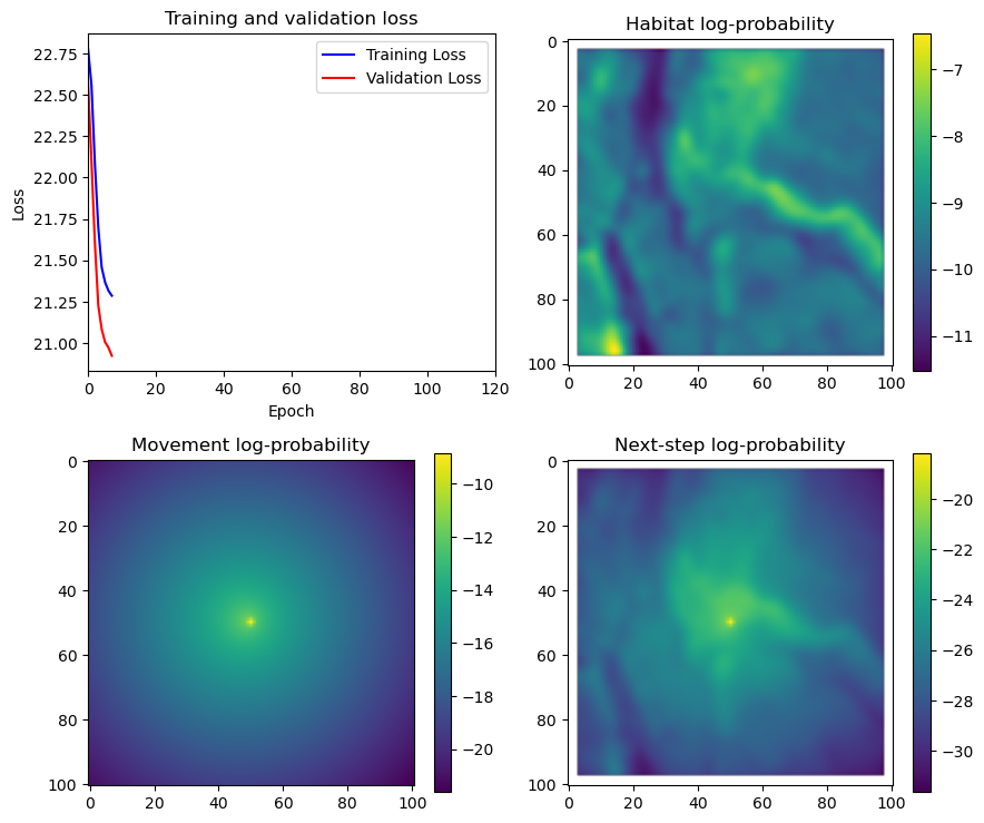
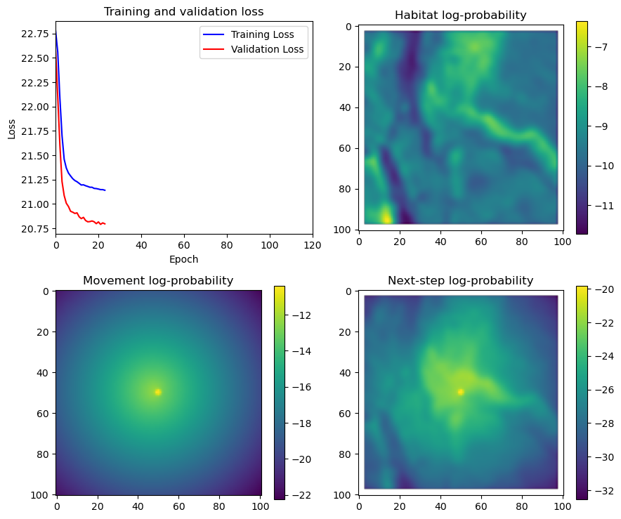
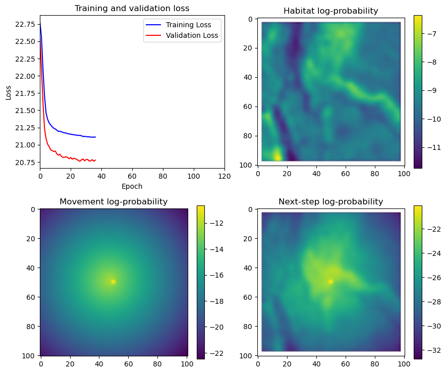
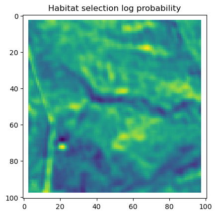
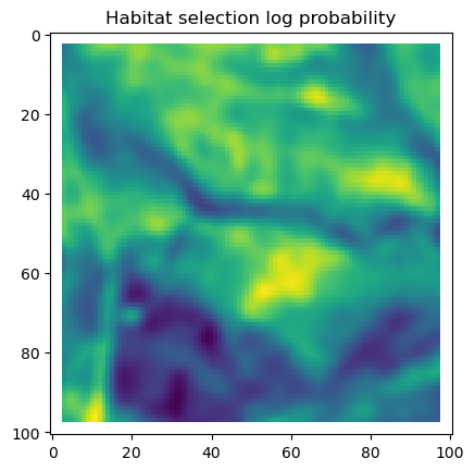
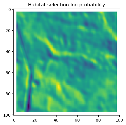
# Plot habitat selection log-probability
im2 = axs_out[0, 1].imshow(hab_density_mask * next_step_mask, cmap='viridis')
axs_out[0, 1].set_title('Habitat selection log-probability')
fig_out.colorbar(im2, ax=axs_out[0, 1], shrink=0.7)
# Movement density log-probability
im3 = axs_out[1, 0].imshow(move_density_mask * next_step_mask, cmap='viridis')
axs_out[1, 0].set_title('Movement log-probability')
fig_out.colorbar(im3, ax=axs_out[1, 0], shrink=0.7)
# Next-step probability
im4 = axs_out[1, 1].imshow(step_density_mask * next_step_mask, cmap='viridis')
axs_out[1, 1].set_title('Next-step log-probability')
fig_out.colorbar(im4, ax=axs_out[1, 1], shrink=0.7)
filename_covs = f'{output_dir}/prediction_images/id{buffalo_id}_step_index{i+1}_yday{yday}_hour{hour_t2}.png'
plt.tight_layout()
plt.savefig(filename_covs, dpi=150) #, bbox_inches='tight'
# plt.show()
plt.close() # Close the figure to free memory